qml.fourier.visualize.radial_box

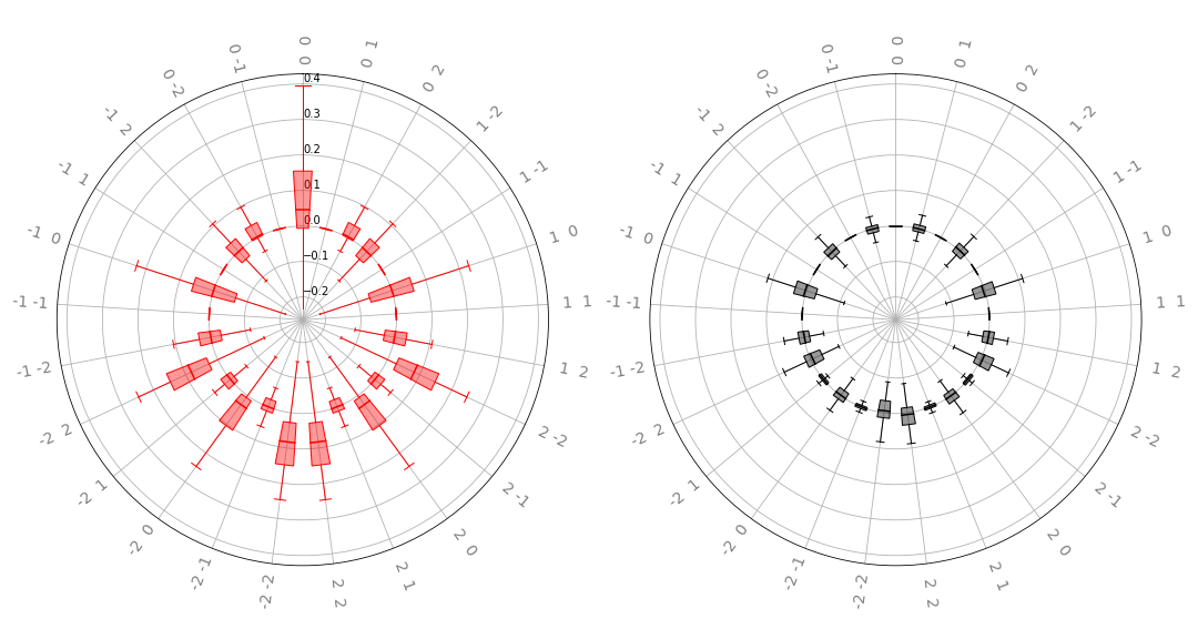
radial_box(coeffs, n_inputs, ax, show_freqs=True, colour_dict=None, show_fliers=True)

Plot a list of sets of Fourier coefficients on a radial plot as box plots.

Produces a 2-panel plot in which the left panel represents the real parts of Fourier coefficients. This method accepts multiple sets of coefficients, and plots the distribution of each coefficient as a boxplot.

Parameters

• coeffs (list[array[complex]]) – A list of sets of Fourier coefficients. The shape of the coefficient arrays should resemble that of the output of numpy/scipy’s fftn function, or coefficients().

• n_inputs (int) – Dimension of the transformed function.

• ax (array[matplotlib.axes.Axes]) – Axes to plot on. For this function, subplots must specify subplot_kw={"polar":True} upon construction.

• show_freqs (bool) – Whether or not to label the frequencies on the radial axis. Turn off for large plots.

• colour_dict (dict[str, str]) – Specify a colour mapping for positive and negative real/imaginary components. If none specified, will default to: {"real" : "red", "imag" : "black"}

• showfliers (bool) – Whether or not to plot outlying “fliers” on the boxplots.

• merge_plots (bool) – Whether to plot real/complex values on the same panel, or on separate panels. Default is to plot real/complex values on separate panels.

Returns

The axes after plotting is complete.

Return type

array[matplotlib.axes.Axes]

Example

Suppose we have the following quantum function:

dev = qml.device('default.qubit', wires=2)

@qml.qnode(dev)
def circuit_with_weights(w, x):
    qml.RX(x[0], wires=0)
    qml.RY(x[1], wires=1)
    qml.CNOT(wires=[1, 0])

    qml.Rot(*w[0], wires=0)
    qml.Rot(*w[1], wires=1)
    qml.CNOT(wires=[1, 0])

    qml.RX(x[0], wires=0)
    qml.RY(x[1], wires=1)
    qml.CNOT(wires=[1, 0])

    return qml.expval(qml.Z(0))

We would like to compute and plot the distribution of Fourier coefficients for many random values of the weights w. First, we generate all the coefficients:

from functools import partial

coeffs = []

n_inputs = 2
degree = 2

for _ in range(100):
    weights = np.random.normal(0, 1, size=(2, 3))
    c = coefficients(partial(circuit_with_weights, weights), n_inputs, degree)
    coeffs.append(c)

We can now plot by setting up a pair of matplotlib axes and passing them to the plotting function. Note that the axes passed must use polar coordinates.

import matplotlib.pyplot as plt
from pennylane.fourier.visualize import radial_box

fig, ax = plt.subplots(
    1, 2, sharex=True, sharey=True,
    subplot_kw={"polar": True},
    figsize=(15, 8)
)

radial_box(coeffs, 2, ax, show_freqs=True, show_fliers=False)

code/api/pennylane.fourier.visualize.radial_box

 

Download Python script

 

Download Notebook

 

View on GitHub