Inspecting circuits
PennyLane offers functionality to inspect, visualize or analyze quantum circuits.
Most of these tools are implemented as transforms. Transforms take a QNode instance and return a function:
>>> @qml.qnode(dev, diff_method='parameter-shift')
... def my_qnode(x, a=True):
...     # ...
>>> new_func = my_transform(qnode)
This new function accepts the same arguments as the QNode and returns the desired outcome, such as a dictionary of the QNode’s properties, a matplotlib figure drawing the circuit, or a DAG representing its connectivity structure.
>>> new_func(0.1, a=False)
More information on the concept of transforms can be found in Di Matteo et al. (2022).
Extracting properties of a circuit
The specs() transform takes a
QNode and creates a function that returns
details about the QNode, including depth, number of gates, and number of
gradient executions required.
For example:
dev = qml.device('default.qubit', wires=4)

@qml.qnode(dev, diff_method='parameter-shift')
def circuit(x, y):
    qml.RX(x[0], wires=0)
    qml.Toffoli(wires=(0, 1, 2))
    qml.CRY(x[1], wires=(0, 1))
    qml.Rot(x[2], x[3], y, wires=0)
    return qml.expval(qml.PauliZ(0)), qml.expval(qml.PauliX(1))
We can now use the specs() transform to generate a function that returns
details and resource information:
>>> x = np.array([0.05, 0.1, 0.2, 0.3], requires_grad=True)
>>> y = np.array(0.4, requires_grad=False)
>>> specs_func = qml.specs(circuit)
>>> specs_func(x, y)
{'resources': Resources(num_wires=3, num_gates=4, gate_types=defaultdict(<class 'int'>, {'RX': 1, 'Toffoli': 1, 'CRY': 1, 'Rot': 1}), depth=4, shots=0),
 'gate_sizes': defaultdict(int, {1: 2, 3: 1, 2: 1}),
 'gate_types': defaultdict(int, {'RX': 1, 'Toffoli': 1, 'CRY': 1, 'Rot': 1}),
 'num_operations': 4,
 'num_observables': 2,
 'num_diagonalizing_gates': 1,
 'num_used_wires': 3,
 'num_trainable_params': 4,
 'depth': 4,
 'num_device_wires': 4,
 'device_name': 'default.qubit',
 'expansion_strategy': 'gradient',
 'gradient_options': {},
 'interface': 'auto',
 'diff_method': 'parameter-shift',
 'gradient_fn': 'pennylane.gradients.parameter_shift.param_shift',
 'num_gradient_executions': 10}
Circuit drawing
PennyLane has two built-in circuit drawers, draw() and
draw_mpl().
For example:
dev = qml.device('lightning.qubit', wires=(0,1,2,3))

@qml.qnode(dev)
def circuit(x, z):
    qml.QFT(wires=(0,1,2,3))
    qml.IsingXX(1.234, wires=(0,2))
    qml.Toffoli(wires=(0,1,2))
    qml.CSWAP(wires=(0,2,3))
    qml.RX(x, wires=0)
    qml.CRZ(z, wires=(3,0))
    return qml.expval(qml.PauliZ(0))


fig, ax = qml.draw_mpl(circuit)(1.2345,1.2345)
fig.show()
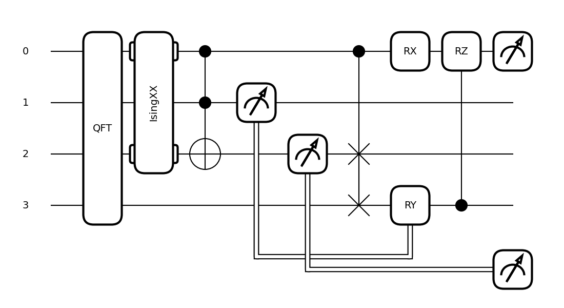
>>> print(qml.draw(circuit)(1.2345,1.2345))
0: ─╭QFT─╭IsingXX(1.23)─╭●─╭●─────RX(1.23)─╭RZ(1.23)─┤  <Z>
1: ─├QFT─│──────────────├●─│───────────────│─────────┤
2: ─├QFT─╰IsingXX(1.23)─╰X─├SWAP───────────│─────────┤
3: ─╰QFT───────────────────╰SWAP───────────╰●────────┤
More information, including various fine-tuning options, can be found in the drawing module.
Debugging with mid-circuit snapshots
When debugging quantum circuits run on simulators, we may want to inspect the current quantum state between gates.
Snapshot is an operator like a gate, but it saves the device state at its location in the circuit instead of manipulating the quantum state.
Currently supported devices include:
default.qubit: each snapshot saves the quantum state vectordefault.mixed: each snapshot saves the density matrixdefault.gaussian: each snapshot saves the covariance matrix and vector of means
During normal execution, the snapshots are ignored:
dev = qml.device("default.qubit", wires=2)

@qml.qnode(dev, interface=None)
def circuit():
    qml.Snapshot(measurement=qml.expval(qml.PauliZ(0)))
    qml.Hadamard(wires=0)
    qml.Snapshot("very_important_state")
    qml.CNOT(wires=[0, 1])
    qml.Snapshot()
    return qml.expval(qml.PauliX(0))
However, when using the snapshots()
transform, intermediate device states will be stored and returned alongside the
results.
>>> qml.snapshots(circuit)()
{0: 1.0,
'very_important_state': array([0.707+0.j, 0.+0.j, 0.707+0.j, 0.+0.j]),
2: array([0.707+0.j, 0.+0.j, 0.+0.j, 0.707+0.j]),
'execution_results': 0.0}
Graph representation
PennyLane makes use of several ways to represent a quantum circuit as a Directed Acyclic Graph (DAG).
DAG of causal relations between ops
A DAG can be used to represent which operator in a circuit is causally related to another. There are two options to construct such a DAG:
The CircuitGraph class takes a list of gates or channels and hermitian observables
as well as a set of wire labels and constructs a DAG in which the Operator
instances are the nodes, and each directed edge corresponds to a wire
(or a group of wires) on which the “nodes” act subsequently.
For example, this can be used to compute the effective depth of a circuit, or to check whether two gates causally influence each other.
import pennylane as qml
from pennylane import CircuitGraph

dev = qml.device('lightning.qubit', wires=(0,1,2,3))

@qml.qnode(dev)
def circuit():
    qml.Hadamard(0)
    qml.CNOT([1, 2])
    qml.CNOT([2, 3])
    qml.CNOT([3, 1])
    return qml.expval(qml.PauliZ(0))


circuit()
tape = circuit.qtape
ops = tape.operations
obs = tape.observables
g = CircuitGraph(ops, obs, tape.wires)
Internally, the CircuitGraph class constructs a rustworkx graph object.
>>> type(g.graph)
<class 'rustworkx.PyDiGraph'>
There is no edge between the Hadamard and the first CNOT, but between consecutive CNOT gates:
>>> g.has_path(ops[0], ops[1])
False
>>> g.has_path(ops[1], ops[3])
True
The Hadamard is connected to the observable, while the CNOT operators are not. The observable
does not follow the Hadamard.
>>> g.has_path(ops[0], obs[0])
True
>>> g.has_path(ops[1], obs[0])
False
>>> g.has_path(obs[0], ops[0])
False
Another way to construct the “causal” DAG of a circuit is to use the
tape_to_graph() function used by the qcut module. This
function takes a quantum tape and creates a MultiDiGraph instance from the networkx python package.
Using the above example, we get:
>>> g2 = qml.qcut.tape_to_graph(tape)
>>> type(g2)
<class 'networkx.classes.multidigraph.MultiDiGraph'>
>>> for k, v in g2.adjacency():
...    print(k, v)
Hadamard(wires=[0]) {expval(Z(0)): {0: {'wire': 0}}}
CNOT(wires=[1, 2]) {CNOT(wires=[2, 3]): {0: {'wire': 2}}, CNOT(wires=[3, 1]): {0: {'wire': 1}}}
CNOT(wires=[2, 3]) {CNOT(wires=[3, 1]): {0: {'wire': 3}}}
CNOT(wires=[3, 1]) {}
expval(Z(0)) {}
DAG of non-commuting ops
The commutation_dag() transform can be used to produce an instance of the CommutationDAG class.
In a commutation DAG, each node represents a quantum operation, and edges represent non-commutation
between two operations.
This transform takes into account that not all operations can be moved next to each other by pairwise commutation:
>>> def circuit(x, y, z):
...     qml.RX(x, wires=0)
...     qml.RX(y, wires=0)
...     qml.CNOT(wires=[1, 2])
...     qml.RY(y, wires=1)
...     qml.Hadamard(wires=2)
...     qml.CRZ(z, wires=[2, 0])
...     qml.RY(-y, wires=1)
...     return qml.expval(qml.PauliZ(0))
>>> dag_fn = qml.commutation_dag(circuit)
>>> dag = dag_fn(np.pi / 4, np.pi / 3, np.pi / 2)
Nodes in the commutation DAG can be accessed via the get_nodes() method, returning a list of
the form (ID, CommutationDAGNode):
>>> nodes = dag.get_nodes()
>>> nodes
NodeDataView({0: <pennylane.transforms.commutation_dag.CommutationDAGNode object at 0x7f461c4bb580>, ...}, data='node')
Specific nodes in the commutation DAG can be accessed via the get_node() method:
>>> second_node = dag.get_node(2)
>>> second_node
<pennylane.transforms.commutation_dag.CommutationDAGNode object at 0x136f8c4c0>
>>> second_node.op
CNOT(wires=[1, 2])
>>> second_node.successors
[3, 4, 5, 6]
>>> second_node.predecessors
[]
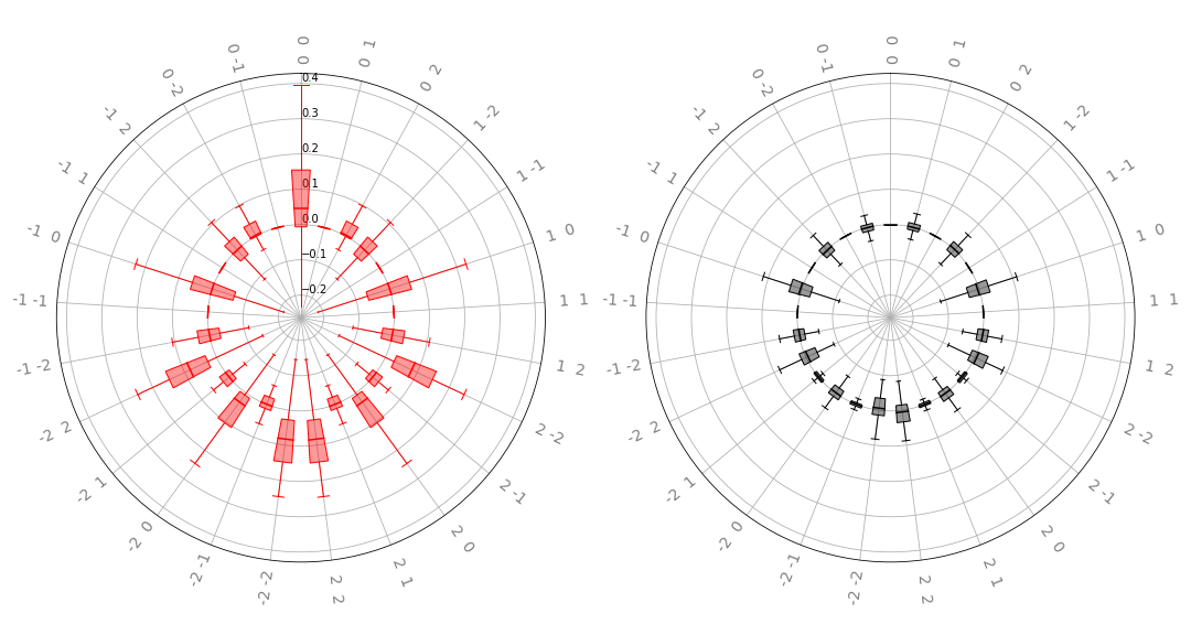
Fourier representation
Parametrized quantum circuits often compute functions in the parameters that can be represented by Fourier series of a low degree.
The qml.fourier module contains functionality to compute and visualize properties of such Fourier series.