Release notes¶
This page contains the release notes for PennyLane.
- orphan
Release 0.35.0 (current release)¶
New features since last release
Qiskit 1.0 integration 🔌
This version of PennyLane makes it easier to import circuits from Qiskit. (#5218) (#5168)
The
qml.from_qiskitfunction converts a Qiskit QuantumCircuit into a PennyLane quantum function. Althoughqml.from_qiskitalready exists in PennyLane, we have made a number of improvements to make importing from Qiskit easier. And yes —qml.from_qiskitfunctionality is compatible with both Qiskit 1.0 and earlier versions! Here’s a comprehensive list of the improvements:You can now append PennyLane measurements onto the quantum function returned by
qml.from_qiskit. Consider this simple Qiskit circuit:import pennylane as qml from qiskit import QuantumCircuit qc = QuantumCircuit(2) qc.rx(0.785, 0) qc.ry(1.57, 1)
We can convert it into a PennyLane QNode in just a few lines, with PennyLane
measurementseasily included:>>> dev = qml.device("default.qubit") >>> measurements = qml.expval(qml.Z(0) @ qml.Z(1)) >>> qfunc = qml.from_qiskit(qc, measurements=measurements) >>> qnode = qml.QNode(qfunc, dev) >>> qnode() tensor(0.00056331, requires_grad=True)
Quantum circuits that already contain Qiskit-side measurements can be faithfully converted with
qml.from_qiskit. Consider this example Qiskit circuit:qc = QuantumCircuit(3, 2) # Teleportation qc.rx(0.9, 0) # Prepare input state on qubit 0 qc.h(1) # Prepare Bell state on qubits 1 and 2 qc.cx(1, 2) qc.cx(0, 1) # Perform teleportation qc.h(0) qc.measure(0, 0) qc.measure(1, 1) with qc.if_test((1, 1)): # Perform first conditional qc.x(2)
This circuit can be converted into PennyLane with the Qiskit measurements still accessible. For example, we can use those results as inputs to a mid-circuit measurement in PennyLane:
@qml.qnode(dev)
def teleport():
    m0, m1 = qml.from_qiskit(qc)()
    qml.cond(m0, qml.Z)(2)
    return qml.density_matrix(2)
>>> teleport()
tensor([[0.81080498+0.j        , 0.        +0.39166345j],
        [0.        -0.39166345j, 0.18919502+0.j        ]], requires_grad=True)
It is now more intuitive to handle and differentiate parametrized Qiskit circuits. Consider the following circuit:
from qiskit.circuit import Parameter
from pennylane import numpy as np

angle0 = Parameter("x")
angle1 = Parameter("y")

qc = QuantumCircuit(2, 2)
qc.rx(angle0, 0)
qc.ry(angle1, 1)
qc.cx(1, 0)
We can convert this circuit into a QNode with two arguments, corresponding to
xandy:measurements = qml.expval(qml.PauliZ(0)) qfunc = qml.from_qiskit(qc, measurements) qnode = qml.QNode(qfunc, dev)
The QNode can be evaluated and differentiated:
>>> x, y = np.array([0.4, 0.5], requires_grad=True)
>>> qnode(x, y)
tensor(0.80830707, requires_grad=True)
>>> qml.grad(qnode)(x, y)
(tensor(-0.34174675, requires_grad=True),
 tensor(-0.44158016, requires_grad=True))
This shows how easy it is to make a Qiskit circuit differentiable with PennyLane.
In addition to circuits, it is also possible to convert operators from Qiskit to PennyLane with a new function called
qml.from_qiskit_op. (#5251)A Qiskit SparsePauliOp can be converted to a PennyLane operator using
qml.from_qiskit_op:>>> from qiskit.quantum_info import SparsePauliOp >>> qiskit_op = SparsePauliOp(["II", "XY"]) >>> qiskit_op SparsePauliOp(['II', 'XY'], coeffs=[1.+0.j, 1.+0.j]) >>> pl_op = qml.from_qiskit_op(qiskit_op) >>> pl_op I(0) + X(1) @ Y(0)
Combined with
qml.from_qiskit, it becomes easy to quickly calculate quantities like expectation values by converting the whole workflow to PennyLane:qc = QuantumCircuit(2) # Create circuit qc.rx(0.785, 0) qc.ry(1.57, 1) measurements = qml.expval(pl_op) # Create QNode qfunc = qml.from_qiskit(qc, measurements) qnode = qml.QNode(qfunc, dev)
>>> qnode()  # Evaluate!
tensor(0.29317504, requires_grad=True)
Native mid-circuit measurements on Default Qubit 💡
Mid-circuit measurements can now be more scalable and efficient in finite-shots mode with
default.qubitby simulating them in a similar way to what happens on quantum hardware. (#5088) (#5120)Previously, mid-circuit measurements (MCMs) would be automatically replaced with an additional qubit using the
@qml.defer_measurementstransform. The circuit below would have required thousands of qubits to simulate.Now, MCMs are performed in a similar way to quantum hardware with finite shots on
default.qubit. For each shot and each time an MCM is encountered, the device evaluates the probability of projecting onto|0>or|1>and makes a random choice to collapse the circuit state. This approach works well when there are a lot of MCMs and the number of shots is not too high.import pennylane as qml dev = qml.device("default.qubit", shots=10) @qml.qnode(dev) def f(): for i in range(1967): qml.Hadamard(0) qml.measure(0) return qml.sample(qml.PauliX(0))
>>> f()
tensor([-1, -1, -1,  1,  1, -1,  1, -1,  1, -1], requires_grad=True)
Work easily and efficiently with operators 🔧
Over the past few releases, PennyLane’s approach to operator arithmetic has been in the process of being overhauled. We have a few objectives:
To make it as easy to work with PennyLane operators as it would be with pen and paper.
To improve the efficiency of operator arithmetic.
The updated operator arithmetic functionality is still being finalized, but can be activated using
qml.operation.enable_new_opmath(). In the next release, the new behaviour will become the default, so we recommend enabling now to become familiar with the new system!The following updates have been made in this version of PennyLane:
You can now easily access Pauli operators via
I,X,Y, andZ: (#5116)>>> from pennylane import I, X, Y, Z >>> X(0) X(0)
The original long-form names
Identity,PauliX,PauliY, andPauliZremain available, but use of the short-form names is now recommended.A new
qml.commutatorfunction is now available that allows you to compute commutators between PennyLane operators. (#5051) (#5052) (#5098)>>> qml.commutator(X(0), Y(0)) 2j * Z(0)
Operators in PennyLane can have a backend Pauli representation, which can be used to perform faster operator arithmetic. Now, the Pauli representation will be automatically used for calculations when available. (#4989) (#5001) (#5003) (#5017) (#5027)
The Pauli representation can be optionally accessed via
op.pauli_rep:>>> qml.operation.enable_new_opmath() >>> op = X(0) + Y(0) >>> op.pauli_rep 1.0 * X(0) + 1.0 * Y(0)
Extensive improvements have been made to the string representations of PennyLane operators, making them shorter and possible to copy-paste as valid PennyLane code. (#5116) (#5138)
>>> 0.5 * X(0)
0.5 * X(0)
>>> 0.5 * (X(0) + Y(1))
0.5 * (X(0) + Y(1))
Sums with many terms are broken up into multiple lines, but can still be copied back as valid code:
>>> 0.5 * (X(0) @ X(1)) + 0.7 * (X(1) @ X(2)) + 0.8 * (X(2) @ X(3))
(
    0.5 * (X(0) @ X(1))
  + 0.7 * (X(1) @ X(2))
  + 0.8 * (X(2) @ X(3))
)
Linear combinations of operators and operator multiplication via
SumandProd, respectively, have been updated to reach feature parity withHamiltonianandTensor, respectively. This should minimize the effort to port over any existing code. (#5070) (#5132) (#5133)Updates include support for grouping via the
paulimodule:>>> obs = [X(0) @ Y(1), Z(0), Y(0) @ Z(1), Y(1)] >>> qml.pauli.group_observables(obs) [[Y(0) @ Z(1)], [X(0) @ Y(1), Y(1)], [Z(0)]]
New Clifford device 🦾
A new
default.clifforddevice enables efficient simulation of large-scale Clifford circuits defined in PennyLane through the use of stim as a backend. (#4936) (#4954) (#5144)Given a circuit with only Clifford gates, one can use this device to obtain the usual range of PennyLane measurements as well as the state represented in the Tableau form of Aaronson & Gottesman (2004):
import pennylane as qml

dev = qml.device("default.clifford", tableau=True)
@qml.qnode(dev)
def circuit():
    qml.CNOT(wires=[0, 1])
    qml.PauliX(wires=[1])
    qml.ISWAP(wires=[0, 1])
    qml.Hadamard(wires=[0])
    return qml.state()
>>> circuit()
array([[0, 1, 1, 0, 0],
      [1, 0, 1, 1, 1],
      [0, 0, 0, 1, 0],
      [1, 0, 0, 1, 1]])
The
default.clifforddevice also supports thePauliError,DepolarizingChannel,BitFlipandPhaseFlipnoise channels when operating in finite-shot mode.
Improvements 🛠
Faster gradients with VJPs and other performance improvements
Vector-Jacobian products (VJPs) can result in faster computations when the output of your quantum Node has a low dimension. They can be enabled by setting
device_vjp=Truewhen loading a QNode. In the next release of PennyLane, VJPs are planned to be used by default, when available.In this release, we have unlocked:
Adjoint device VJPs can be used with
jax.jacobian, meaning thatdevice_vjp=Trueis always faster when using JAX withdefault.qubit. (#4963)PennyLane can now use lightning-provided VJPs. (#4914)
VJPs can be used with TensorFlow, though support has not yet been added for
tf.Functionand Tensorflow Autograph. (#4676)
Measuring
qml.probsis now faster due to an optimization in converting samples to counts. (#5145)The performance of circuit-cutting workloads with large numbers of generated tapes has been improved. (#5005)
Queueing (
AnnotatedQueue) has been removed fromqml.cut_circuitandqml.cut_circuit_mcto improve performance for large workflows. (#5108)
Community contributions 🥳
A new function called
qml.fermi.parity_transformhas been added for parity mapping of a fermionic Hamiltonian. (#4928)It is now possible to transform a fermionic Hamiltonian to a qubit Hamiltonian with parity mapping.
import pennylane as qml
fermi_ham = qml.fermi.FermiWord({(0, 0) : '+', (1, 1) : '-'})

qubit_ham = qml.fermi.parity_transform(fermi_ham, n=6)
>>> print(qubit_ham)
-0.25j * Y(0) + (-0.25+0j) * (X(0) @ Z(1)) + (0.25+0j) * X(0) + 0.25j * (Y(0) @ Z(1))
The transform
split_non_commutingnow accepts measurements of typeprobs,sample, andcounts, which accept both wires and observables. (#4972)The efficiency of matrix calculations when an operator is symmetric over a given set of wires has been improved. (#3601)
The
pennylane/math/quantum.pymodule now has support for computing the minimum entropy of a density matrix. (#3959)>>> x = [1, 0, 0, 1] / np.sqrt(2) >>> x = qml.math.dm_from_state_vector(x) >>> qml.math.min_entropy(x, indices=[0]) 0.6931471805599455
A function called
apply_operationthat applies operations to device-compatible states has been added to the newqutrit_mixedmodule found inqml.devices. (#5032)A function called
measurehas been added to the newqutrit_mixedmodule found inqml.devicesthat measures device-compatible states for a collection of measurement processes. (#5049)A
partial_tracefunction has been added toqml.mathfor taking the partial trace of matrices. (#5152)
Other operator arithmetic improvements
The following capabilities have been added for Pauli arithmetic: (#4989) (#5001) (#5003) (#5017) (#5027) (#5018)
You can now multiply
PauliWordandPauliSentenceinstances by scalars (e.g.,0.5 * PauliWord({0: "X"})or0.5 * PauliSentence({PauliWord({0: "X"}): 1.})).You can now intuitively add and subtract
PauliWordandPauliSentenceinstances and scalars together (scalars are treated implicitly as multiples of the identity,I). For example,ps1 + pw1 + 1.for some Pauli wordpw1 = PauliWord({0: "X", 1: "Y"})and Pauli sentenceps1 = PauliSentence({pw1: 3.}).You can now element-wise multiply
PauliWord,PauliSentence, and operators together withqml.dot(e.g.,qml.dot([0.5, -1.5, 2], [pw1, ps1, id_word])withid_word = PauliWord({})).qml.matrixnow acceptsPauliWordandPauliSentenceinstances (e.g.,qml.matrix(PauliWord({0: "X"}))).It is now possible to compute commutators with Pauli operators natively with the new
commutatormethod.>>> op1 = PauliWord({0: "X", 1: "X"}) >>> op2 = PauliWord({0: "Y"}) + PauliWord({1: "Y"}) >>> op1.commutator(op2) 2j * Z(0) @ X(1) + 2j * X(0) @ Z(1)
Composite operations (e.g., those made with
qml.prodandqml.sum) and scalar-product operations convertHamiltonianandTensoroperands toSumandProdtypes, respectively. This helps avoid the mixing of incompatible operator types. (#5031) (#5063)qml.Identity()can be initialized without wires. Measuring it is currently not possible, though. (#5106)qml.dotnow returns aSumclass even when all the coefficients match. (#5143)qml.pauli.group_observablesnow supports groupingProdandSProdoperators. (#5070)The performance of converting a
PauliSentenceto aSumhas been improved. (#5141) (#5150)Akin to
qml.Hamiltonianfeatures, the coefficients and operators that make up composite operators formed viaSumorProdcan now be accessed with theterms()method. (#5132) (#5133) (#5164)>>> qml.operation.enable_new_opmath() >>> op = X(0) @ (0.5 * X(1) + X(2)) >>> op.terms() ([0.5, 1.0], [X(1) @ X(0), X(2) @ X(0)])
String representations of
ParametrizedHamiltonianhave been updated to match the style of other PL operators. (#5215)
Other improvements
The
pl-device-testsuite is now compatible with theqml.devices.Deviceinterface. (#5229)The
QSVToperation now determines itsdatafrom the block encoding and projector operator data. (#5226) (#5248)The
BlockEncodeoperator is now JIT-compatible with JAX. (#5110)The
qml.qsvtfunction usesqml.GlobalPhaseinstead ofqml.expto define a global phase. (#5105)The
tests/ops/functions/conftest.pytest has been updated to ensure that all operator types are tested for validity. (#4978)A new
pennylane.workflowmodule has been added. This module now containsqnode.py,execution.py,set_shots.py,jacobian_products.py, and the submoduleinterfaces. (#5023)A more informative error is now raised when calling
adjoint_jacobianwith trainable state-prep operations. (#5026)qml.workflow.get_transform_programandqml.workflow.construct_batchhave been added to inspect the transform program and batch of tapes at different stages. (#5084)All custom controlled operations such as
CRX,CZ,CNOT,ControlledPhaseShiftnow inherit fromControlledOp, giving them additional properties such ascontrol_wireandcontrol_values. Callingqml.ctrlonRX,RY,RZ,Rot, andPhaseShiftwith a single control wire will return gates of typesCRX,CRY, etc. as opposed to a generalControlledoperator. (#5069) (#5199)The CI will now fail if coverage data fails to upload to codecov. Previously, it would silently pass and the codecov check itself would never execute. (#5101)
qml.ctrlcalled on operators with custom controlled versions will now return instances of the custom class, and it will flatten nested controlled operators to a single multi-controlled operation. ForPauliX,CNOT,Toffoli, andMultiControlledX, callingqml.ctrlwill always resolve to the best option inCNOT,Toffoli, orMultiControlledXdepending on the number of control wires and control values. (#5125)Unwanted warning filters have been removed from tests and no
PennyLaneDeprecationWarnings are being raised unexpectedly. (#5122)New error tracking and propagation functionality has been added (#5115) (#5121)
The method
map_batch_transformhas been replaced with the method_batch_transformimplemented inTransformDispatcher. (#5212)TransformDispatchercan now dispatch onto a batch of tapes, making it easier to compose transforms when working in the tape paradigm. (#5163)qml.ctrlis now a simple wrapper that either calls PennyLane’s built increate_controlled_opor uses the Catalyst implementation. (#5247)Controlled composite operations can now be decomposed using ZYZ rotations. (#5242)
New functions called
qml.devices.modifiers.simulator_trackingandqml.devices.modifiers.single_tape_supporthave been added to add basic default behavior onto a device class. (#5200)
Breaking changes 💔
Passing additional arguments to a transform that decorates a QNode must now be done through the use of
functools.partial. (#5046)qml.ExpvalCosthas been removed. Users should useqml.expval()moving forward. (#5097)Caching of executions is now turned off by default when
max_diff == 1, as the classical overhead cost outweighs the probability that duplicate circuits exists. (#5243)The entry point convention registering compilers with PennyLane has changed. (#5140)
To allow for packages to register multiple compilers with PennyLane, the
entry_pointsconvention under the designated group namepennylane.compilershas been modified.Previously, compilers would register
qjit(JIT decorator),ops(compiler-specific operations), andcontext(for tracing and program capture).Now, compilers must register
compiler_name.qjit,compiler_name.ops, andcompiler_name.context, wherecompiler_nameis replaced by the name of the provided compiler.For more information, please see the documentation on adding compilers.
PennyLane source code is now compatible with the latest version of
black. (#5112) (#5119)gradient_analysis_and_validationhas been renamed tofind_and_validate_gradient_methods. Instead of returning a list, it now returns a dictionary of gradient methods for each parameter index, and no longer mutates the tape. (#5035)Multiplying two
PauliWordinstances no longer returns a tuple(new_word, coeff)but insteadPauliSentence({new_word: coeff}). The old behavior is still available with the private methodPauliWord._matmul(other)for faster processing. (#5045)Observable.return_typehas been removed. Instead, you should inspect the type of the surrounding measurement process. (#5044)ClassicalShadow.entropy()no longer needs anatolkeyword as a better method to estimate entropies from approximate density matrix reconstructions (with potentially negative eigenvalues). (#5048)Controlled operators with a custom controlled version decompose like how their controlled counterpart decomposes as opposed to decomposing into their controlled version. (#5069) (#5125)
For example:
>>> qml.ctrl(qml.RX(0.123, wires=1), control=0).decomposition()
[
  RZ(1.5707963267948966, wires=[1]),
  RY(0.0615, wires=[1]),
  CNOT(wires=[0, 1]),
  RY(-0.0615, wires=[1]),
  CNOT(wires=[0, 1]),
  RZ(-1.5707963267948966, wires=[1])
]
QuantumScript.is_sampledandQuantumScript.all_sampledhave been removed. Users should now validate these properties manually. (#5072)qml.transforms.one_qubit_decompositionandqml.transforms.two_qubit_decompositionhave been removed. Instead, you should useqml.ops.one_qubit_decompositionandqml.ops.two_qubit_decomposition. (#5091)
Deprecations 👋
Calling
qml.matrixwithout providing awire_orderon objects where the wire order could be ambiguous now raises a warning. In the future, thewire_orderargument will be required in these cases. (#5039)Operator.validate_subspace(subspace)has been relocated to theqml.ops.qutrit.parametric_opsmodule and will be removed from the Operator class in an upcoming release. (#5067)Matrix and tensor products between
PauliWordandPauliSentenceinstances are done using the@operator,*will be used only for scalar multiplication. Note also the breaking change that the product of twoPauliWordinstances now returns aPauliSentenceinstead of a tuple(new_word, coeff). (#4989) (#5054)MeasurementProcess.nameandMeasurementProcess.dataare now deprecated, as they contain dummy values that are no longer needed. (#5047) (#5071) (#5076) (#5122)qml.pauli.pauli_multandqml.pauli.pauli_mult_with_phaseare now deprecated. Instead, you should useqml.simplify(qml.prod(pauli_1, pauli_2))to get the reduced operator. (#5057)The private functions
_pauli_mult,_binary_matrixand_get_pauli_mapfrom thepaulimodule have been deprecated, as they are no longer used anywhere and the same functionality can be achieved using newer features in thepaulimodule. (#5057)Sum.ops,Sum.coeffs,Prod.opsandProd.coeffswill be deprecated in the future. (#5164)
Documentation 📝
The module documentation for
pennylane.tapenow explains the difference betweenQuantumTapeandQuantumScript. (#5065)A typo in a code example in the
qml.transformsAPI has been fixed. (#5014)Documentation for
qml.datahas been updated and now mentions a way to access the same dataset simultaneously from multiple environments. (#5029)A clarification for the definition of
argnumadded to gradient methods has been made. (#5035)A typo in the code example for
qml.qchem.dipole_ofhas been fixed. (#5036)A development guide on deprecations and removals has been added. (#5083)
A note about the eigenspectrum of second-quantized Hamiltonians has been added to
qml.eigvals. (#5095)A warning about two mathematically equivalent Hamiltonians undergoing different time evolutions has been added to
qml.TrotterProductandqml.ApproxTimeEvolution. (#5137)A reference to the paper that provides the image of the
qml.QAOAEmbeddingtemplate has been added. (#5130)The docstring of
qml.samplehas been updated to advise the use of single-shot expectations instead when differentiating a circuit. (#5237)A quick start page has been added called “Importing Circuits”. This explains how to import quantum circuits and operations defined outside of PennyLane. (#5281)
Bug fixes 🐛
QubitChannelcan now be used with jitting. (#5288)Fixed a bug in the matplotlib drawer where the colour of
Barrierdid not match the requested style. (#5276)qml.drawandqml.draw_mplnow apply all applied transforms before drawing. (#5277)ctrl_decomp_zyzis now differentiable. (#5198)qml.ops.Pow.matrix()is now differentiable with TensorFlow with integer exponents. (#5178)The
qml.MottonenStatePreparationtemplate has been updated to include a global phase operation. (#5166)Fixed a queuing bug when using
qml.prodwith a quantum function that queues a single operator. (#5170)The
qml.TrotterProducttemplate has been updated to accept scalar products of operators as an input Hamiltonian. (#5073)Fixed a bug where caching together with JIT compilation and broadcasted tapes yielded wrong results
Operator.hashnow depends on the memory location,id, of a JAX tracer instead of its string representation. (#3917)qml.transforms.undo_swapscan now work with operators with hyperparameters or nesting. (#5081)qml.transforms.split_non_commutingwill now pass the original shots along. (#5081)If
argnumis provided to a gradient transform, only the parameters specified inargnumwill have their gradient methods validated. (#5035)StatePrepoperations expanded onto more wires are now compatible with backprop. (#5028)qml.equalworks well withqml.Sumoperators when wire labels are a mix of integers and strings. (#5037)The return value of
Controlled.generatornow contains a projector that projects onto the correct subspace based on the control value specified. (#5068)CosineWindowno longer raises an unexpected error when used on a subset of wires at the beginning of a circuit. (#5080)tf.functionnow works withTensorSpec(shape=None)by skipping batch size computation. (#5089)PauliSentence.wiresno longer imposes a false order. (#5041)qml.qchem.import_statenow applies the chemist-to-physicist sign convention when initializing a PennyLane state vector from classically pre-computed wavefunctions. That is, it interleaves spin-up/spin-down operators for the same spatial orbital index, as standard in PennyLane (instead of commuting all spin-up operators to the left, as is standard in quantum chemistry). (#5114)Multi-wire controlled
CNOTandPhaseShiftare now be decomposed correctly. (#5125) (#5148)draw_mplno longer raises an error when drawing a circuit containing an adjoint of a controlled operation. (#5149)default.mixedno longer throwsValueErrorwhen applying a state vector that is not of typecomplex128when used with tensorflow. (#5155)ctrl_decomp_zyzno longer raises aTypeErrorif the rotation parameters are of typetorch.Tensor(#5183)Comparing
ProdandSumobjects now works regardless of nested structure withqml.equalif the operators have a validpauli_repproperty. (#5177)Controlled
GlobalPhasewith non-zero control wires no longer throws an error. (#5194)A
QNodetransformed withmitigate_with_znenow accepts batch parameters. (#5195)The matrix of an empty
PauliSentenceinstance is now correct (all-zeros). Further, matrices of emptyPauliWordandPauliSentenceinstances can now be turned into matrices. (#5188)PauliSentenceinstances can handle matrix multiplication withPauliWordinstances. (#5208)CompositeOp.eigendecompositionis now JIT-compatible. (#5207)QubitDensityMatrixnow works with JAX-JIT on thedefault.mixeddevice. (#5203) (#5236)When a QNode specifies
diff_method="adjoint",default.qubitno longer tries to decompose non-trainable operations with non-scalar parameters such asQubitUnitary. (#5233)The overwriting of the class names of
I,X,Y, andZno longer happens in the initialization after causing problems with datasets. This now happens globally. (#5252)The
adjoint_metric_tensortransform now works withjax. (#5271)
Contributors ✍️
This release contains contributions from (in alphabetical order):
Abhishek Abhishek, Mikhail Andrenkov, Utkarsh Azad, Trenten Babcock, Gabriel Bottrill, Thomas Bromley, Astral Cai, Skylar Chan, Isaac De Vlugt, Diksha Dhawan, Lillian Frederiksen, Pietropaolo Frisoni, Eugenio Gigante, Diego Guala, David Ittah, Soran Jahangiri, Jacky Jiang, Korbinian Kottmann, Christina Lee, Xiaoran Li, Vincent Michaud-Rioux, Romain Moyard, Pablo Antonio Moreno Casares, Erick Ochoa Lopez, Lee J. O’Riordan, Mudit Pandey, Alex Preciado, Matthew Silverman, Jay Soni.
- orphan
Release 0.34.0¶
New features since last release
Statistics and drawing for mid-circuit measurements 🎨
It is now possible to return statistics of composite mid-circuit measurements. (#4888)
Mid-circuit measurement results can be composed using basic arithmetic operations and then statistics can be calculated by putting the result within a PennyLane measurement like
qml.expval(). For example:import pennylane as qml dev = qml.device("default.qubit") @qml.qnode(dev) def circuit(phi, theta): qml.RX(phi, wires=0) m0 = qml.measure(wires=0) qml.RY(theta, wires=1) m1 = qml.measure(wires=1) return qml.expval(~m0 + m1) print(circuit(1.23, 4.56))
1.2430187928114291Another option, for ease-of-use when using
qml.sample(),qml.probs(), orqml.counts(), is to provide a simple list of mid-circuit measurement results:dev = qml.device("default.qubit") @qml.qnode(dev) def circuit(phi, theta): qml.RX(phi, wires=0) m0 = qml.measure(wires=0) qml.RY(theta, wires=1) m1 = qml.measure(wires=1) return qml.sample(op=[m0, m1]) print(circuit(1.23, 4.56, shots=5))
[[0 1]
 [0 1]
 [0 0]
 [1 0]
 [0 1]]
Composite mid-circuit measurement statistics are supported on
default.qubitanddefault.mixed. To learn more about which measurements and arithmetic operators are supported, refer to the measurements page and the documentation for qml.measure.Mid-circuit measurements can now be visualized with the text-based
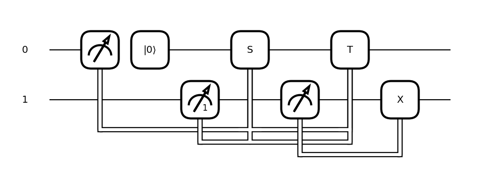
qml.draw()and the graphicalqml.draw_mpl()methods. (#4775) (#4803) (#4832) (#4901) (#4850) (#4917) (#4930) (#4957)Drawing of mid-circuit measurement capabilities including qubit reuse and reset, postselection, conditioning, and collecting statistics is now supported. Here is an all-encompassing example:
def circuit():
    m0 = qml.measure(0, reset=True)
    m1 = qml.measure(1, postselect=1)
    qml.cond(m0 - m1 == 0, qml.S)(0)
    m2 = qml.measure(1)
    qml.cond(m0 + m1 == 2, qml.T)(0)
    qml.cond(m2, qml.PauliX)(1)
The text-based drawer outputs:
>>> print(qml.draw(circuit)())
0: ──┤↗│  │0⟩────────S───────T────┤
1: ───║────────┤↗₁├──║──┤↗├──║──X─┤
      ╚═════════║════╬═══║═══╣  ║
                ╚════╩═══║═══╝  ║
                         ╚══════╝
The graphical drawer outputs:
>>> print(qml.draw_mpl(circuit)())
Catalyst is seamlessly integrated with PennyLane ⚗️
Catalyst, our next-generation compilation framework, is now accessible within PennyLane, allowing you to more easily benefit from hybrid just-in-time (JIT) compilation.
To access these features, simply install
pennylane-catalyst:pip install pennylane-catalyst
The qml.compiler module provides support for hybrid quantum-classical compilation. (#4692) (#4979)
Through the use of the
qml.qjitdecorator, entire workflows can be JIT compiled — including both quantum and classical processing — down to a machine binary on first-function execution. Subsequent calls to the compiled function will execute the previously-compiled binary, resulting in significant performance improvements.import pennylane as qml dev = qml.device("lightning.qubit", wires=2) @qml.qjit @qml.qnode(dev) def circuit(theta): qml.Hadamard(wires=0) qml.RX(theta, wires=1) qml.CNOT(wires=[0,1]) return qml.expval(qml.PauliZ(wires=1))
>>> circuit(0.5)  # the first call, compilation occurs here
array(0.)
>>> circuit(0.5)  # the precompiled quantum function is called
array(0.)
Currently, PennyLane supports the Catalyst hybrid compiler with the
qml.qjitdecorator. A significant benefit of Catalyst is the ability to preserve complex control flow around quantum operations — such asifstatements andforloops, and including measurement feedback — during compilation, while continuing to support end-to-end autodifferentiation.The following functions can now be used with the
qml.qjitdecorator:qml.grad,qml.jacobian,qml.vjp,qml.jvp, andqml.adjoint. (#4709) (#4724) (#4725) (#4726)When
qml.gradorqml.jacobianare used with@qml.qjit, they are patched to catalyst.grad and catalyst.jacobian, respectively.dev = qml.device("lightning.qubit", wires=1) @qml.qjit def workflow(x): @qml.qnode(dev) def circuit(x): qml.RX(np.pi * x[0], wires=0) qml.RY(x[1], wires=0) return qml.probs() g = qml.jacobian(circuit) return g(x)
>>> workflow(np.array([2.0, 1.0]))
array([[ 3.48786850e-16, -4.20735492e-01],
       [-8.71967125e-17,  4.20735492e-01]])
JIT-compatible functionality for control flow has been added via
qml.for_loop,qml.while_loop, andqml.cond. (#4698) (#5006)qml.for_loopandqml.while_loopcan be deployed as decorators on functions that are the body of the loop. The arguments to both follow typical conventions:@qml.for_loop(lower_bound, upper_bound, step)
@qml.while_loop(cond_function)
Here is a concrete example with
qml.for_loop:qml.for_loopandqml.while_loopcan be deployed as decorators on functions that are the body of the loop. The arguments to both follow typical conventions:@qml.for_loop(lower_bound, upper_bound, step)
@qml.while_loop(cond_function)
Here is a concrete example with
qml.for_loop:dev = qml.device("lightning.qubit", wires=1) @qml.qjit @qml.qnode(dev) def circuit(n: int, x: float): @qml.for_loop(0, n, 1) def loop_rx(i, x): # perform some work and update (some of) the arguments qml.RX(x, wires=0) # update the value of x for the next iteration return jnp.sin(x) # apply the for loop final_x = loop_rx(x) return qml.expval(qml.PauliZ(0)), final_x
>>> circuit(7, 1.6)
(array(0.97926626), array(0.55395718))
Decompose circuits into the Clifford+T gateset 🧩
The new
qml.clifford_t_decomposition()transform provides an approximate breakdown of an input circuit into the Clifford+T gateset. Behind the scenes, this decomposition is enacted via thesk_decomposition()function using the Solovay-Kitaev algorithm. (#4801) (#4802)The Solovay-Kitaev algorithm approximately decomposes a quantum circuit into the Clifford+T gateset. To account for this, a desired total circuit decomposition error,
epsilon, must be specified when usingqml.clifford_t_decomposition:dev = qml.device("default.qubit") @qml.qnode(dev) def circuit(): qml.RX(1.1, 0) return qml.state() circuit = qml.clifford_t_decomposition(circuit, epsilon=0.1)
>>> print(qml.draw(circuit)())
0: ──T†──H──T†──H──T──H──T──H──T──H──T──H──T†──H──T†──T†──H──T†──H──T──H──T──H──T──H──T──H──T†──H

───T†──H──T──H──GlobalPhase(0.39)─┤
The resource requirements of this circuit can also be evaluated:
>>> with qml.Tracker(dev) as tracker:
...     circuit()
>>> resources_lst = tracker.history["resources"]
>>> resources_lst[0]
wires: 1
gates: 34
depth: 34
shots: Shots(total=None)
gate_types:
{'Adjoint(T)': 8, 'Hadamard': 16, 'T': 9, 'GlobalPhase': 1}
gate_sizes:
{1: 33, 0: 1}
Use an iterative approach for quantum phase estimation 🔄
Iterative Quantum Phase Estimation is now available with
qml.iterative_qpe. (#4804)The subroutine can be used similarly to mid-circuit measurements:
import pennylane as qml

dev = qml.device("default.qubit", shots=5)

@qml.qnode(dev)
def circuit():

  # Initial state
  qml.PauliX(wires=[0])

  # Iterative QPE
  measurements = qml.iterative_qpe(qml.RZ(2., wires=[0]), ancilla=[1], iters=3)

  return [qml.sample(op=meas) for meas in measurements]
>>> print(circuit())
[array([0, 0, 0, 0, 0]), array([1, 0, 0, 0, 0]), array([0, 1, 1, 1, 1])]
The \(i\)-th element in the list refers to the 5 samples generated by the \(i\)-th measurement of the algorithm.
Improvements 🛠
Community contributions 🥳
The
+=operand can now be used with aPauliSentence, which has also provides a performance boost. (#4662)The Approximate Quantum Fourier Transform (AQFT) is now available with
qml.AQFT. (#4715)qml.drawandqml.draw_mplnow render operator IDs. (#4749)The ID can be specified as a keyword argument when instantiating an operator:
>>> def circuit():
...     qml.RX(0.123, id="data", wires=0)
>>> print(qml.draw(circuit)())
0: ──RX(0.12,"data")─┤
Non-parametric operators such as
Barrier,Snapshot, andWirecuthave been grouped together and moved topennylane/ops/meta.py. Additionally, the relevant tests have been organized and placed in a new file,tests/ops/test_meta.py. (#4789)The
TRX,TRY, andTRZoperators are now differentiable via backpropagation ondefault.qutrit. (#4790)The function
qml.equalnow supportsControlledSequenceoperators. (#4829)XZX decomposition has been added to the list of supported single-qubit unitary decompositions. (#4862)
==and!=operands can now be used withTransformProgramandTransformContainersinstances. (#4858)A
qutrit_mixedmodule has been added toqml.devicesto store helper functions for a future qutrit mixed-state device. A function calledcreate_initial_statehas been added to this module that creates device-compatible initial states. (#4861)The function
qml.Snapshotnow supports arbitrary state-based measurements (i.e., measurements of typeStateMeasurement). (#4876)qml.equalnow supports the comparison ofQuantumScriptandBasisRotationobjects. (#4902) (#4919)The function
qml.draw_mplnow accept a keyword argumentfigto specify the output figure window. (#4956)
Better support for batching
qml.AmplitudeEmbeddingnow supports batching when used with Tensorflow. (#4818)default.qubitcan now evolve already batched states withqml.pulse.ParametrizedEvolution. (#4863)qml.ArbitraryUnitarynow supports batching. (#4745)Operator and tape batch sizes are evaluated lazily, helping run expensive computations less frequently and an issue with Tensorflow pre-computing batch sizes. (#4911)
Performance improvements and benchmarking
Autograd, PyTorch, and JAX can now use vector-Jacobian products (VJPs) provided by the device from the new device API. If a device provides a VJP, this can be selected by providing
device_vjp=Trueto a QNode orqml.execute. (#4935) (#4557) (#4654) (#4878) (#4841)>>> dev = qml.device('default.qubit') >>> @qml.qnode(dev, diff_method="adjoint", device_vjp=True) >>> def circuit(x): ... qml.RX(x, wires=0) ... return qml.expval(qml.PauliZ(0)) >>> with dev.tracker: ... g = qml.grad(circuit)(qml.numpy.array(0.1)) >>> dev.tracker.totals {'batches': 1, 'simulations': 1, 'executions': 1, 'vjp_batches': 1, 'vjps': 1} >>> g -0.09983341664682815
qml.expvalwith largeHamiltonianobjects is now faster and has a significantly lower memory footprint (and constant with respect to the number ofHamiltonianterms) when theHamiltonianis aPauliSentence. This is due to the introduction of a specializeddotmethod in thePauliSentenceclass which performsPauliSentence-stateproducts. (#4839)default.qubitno longer uses a dense matrix forMultiControlledXfor more than 8 operation wires. (#4673)Some relevant Pytests have been updated to enable its use as a suite of benchmarks. (#4703)
default.qubitnow appliesGroverOperatorfaster by not using its matrix representation but a custom rule forapply_operation. Also, the matrix representation ofGroverOperatornow runs faster. (#4666)A new pipeline to run benchmarks and plot graphs comparing with a fixed reference has been added. This pipeline will run on a schedule and can be activated on a PR with the label
ci:run_benchmarks. (#4741)default.qubitnow supports adjoint differentiation for arbitrary diagonal state-based measurements. (#4865)The benchmarks pipeline has been expanded to export all benchmark data to a single JSON file and a CSV file with runtimes. This includes all references and local benchmarks. (#4873)
Final phase of updates to transforms
qml.quantum_monte_carloandqml.simplifynow use the new transform system. (#4708) (#4949)The formal requirement that type hinting be provided when using the
qml.transformdecorator has been removed. Type hinting can still be used, but is now optional. Please use a type checker such as mypy if you wish to ensure types are being passed correctly. (#4942)
Other improvements
Add PyTree-serialization interface for the
Wiresclass. (#4998)PennyLane now supports Python 3.12. (#4985)
SampleMeasurementnow has an optional methodprocess_countsfor computing the measurement results from a counts dictionary. (#4941)A new function called
ops.functions.assert_validhas been added for checking if anOperatorclass is defined correctly. (#4764)Shotsobjects can now be multiplied by scalar values. (#4913)GlobalPhasenow decomposes to nothing in case devices do not support global phases. (#4855)Custom operations can now provide their matrix directly through the
Operator.matrix()method without needing to update thehas_matrixproperty.has_matrixwill now automatically beTrueifOperator.matrixis overridden, even ifOperator.compute_matrixis not. (#4844)The logic for re-arranging states before returning them has been improved. (#4817)
When multiplying
SparseHamiltonians by a scalar value, the result now stays as aSparseHamiltonian. (#4828)trainable_paramscan now be set upon initialization of aQuantumScriptinstead of having to set the parameter after initialization. (#4877)default.qubitnow calculates the expectation value ofHermitianoperators in a differentiable manner. (#4866)The
rotdecomposition now has support for returning a global phase. (#4869)The
"pennylane_sketch"MPL-drawer style has been added. This is the same as the"pennylane"style, but with sketch-style lines. (#4880)Operators now define a
pauli_repproperty, an instance ofPauliSentence, defaulting toNoneif the operator has not defined it (or has no definition in the Pauli basis). (#4915)qml.ShotAdaptiveOptimizercan now use a multinomial distribution for spreading shots across the terms of a Hamiltonian measured in a QNode. Note that this is equivalent to what can be done withqml.ExpvalCost, but this is the preferred method becauseExpvalCostis deprecated. (#4896)Decomposition of
qml.PhaseShiftnow usesqml.GlobalPhasefor retaining the global phase information. (#4657) (#4947)qml.equalforControlledoperators no longer returnsFalsewhen equivalent but differently-ordered sets of control wires and control values are compared. (#4944)All PennyLane
Operatorsubclasses are automatically tested byops.functions.assert_validto ensure that they follow PennyLaneOperatorstandards. (#4922)Probability measurements can now be calculated from a
countsdictionary with the addition of aprocess_countsmethod in theProbabilityMPclass. (#4952)ClassicalShadow.entropynow uses the algorithm outlined in 1106.5458 to project the approximate density matrix (with potentially negative eigenvalues) onto the closest valid density matrix. (#4959)The
ControlledSequence.compute_decompositiondefault now decomposes thePowoperators, improving compatibility with machine learning interfaces. (#4995)
Breaking changes 💔
The function
qml.transforms.classical_jacobianhas been moved to the gradients module and is now accessible asqml.gradients.classical_jacobian. (#4900)The transforms submodule
qml.transforms.qcutis now its own module:qml.qcut. (#4819)The decomposition of
GroverOperatornow has an additional global phase operation. (#4666)qml.condand theConditionaloperation have been moved from thetransformsfolder to theops/op_mathfolder.qml.transforms.Conditionalwill now be available asqml.ops.Conditional. (#4860)The
prepkeyword argument has been removed fromQuantumScriptandQuantumTape.StatePrepBaseoperations should be placed at the beginning of theopslist instead. (#4756)qml.gradients.pulse_generatoris now namedqml.gradients.pulse_odegento adhere to paper naming conventions. (#4769)Specifying
control_valuespassed toqml.ctrlas a string is no longer supported. (#4816)The
rotdecomposition will now normalize its rotation angles to the range[0, 4pi]for consistency (#4869)QuantumScript.graphis now built usingtape.measurementsinstead oftape.observablesbecause it depended on the now-deprecatedObservable.return_typeproperty. (#4762)The
"pennylane"MPL-drawer style now draws straight lines instead of sketch-style lines. (#4880)The default value for the
term_samplingargument ofShotAdaptiveOptimizeris nowNoneinstead of"weighted_random_sampling". (#4896)
Deprecations 👋
single_tape_transform,batch_transform,qfunc_transform, andop_transformare deprecated. Use the newqml.transformfunction instead. (#4774)Observable.return_typeis deprecated. Instead, you should inspect the type of the surrounding measurement process. (#4762) (#4798)All deprecations now raise a
qml.PennyLaneDeprecationWarninginstead of aUserWarning. (#4814)QuantumScript.is_sampledandQuantumScript.all_sampledare deprecated. Users should now validate these properties manually. (#4773)With an algorithmic improvement to
ClassicalShadow.entropy, the keywordatolbecomes obsolete and will be removed in v0.35. (#4959)
Documentation 📝
Documentation for unitaries and operations’ decompositions has been moved from
qml.transformstoqml.ops.ops_math. (#4906)Documentation for
qml.metric_tensorandqml.adjoint_metric_tensorandqml.transforms.classical_jacobianis now accessible via the gradients API pageqml.gradientsin the documentation. (#4900)Documentation for
qml.specshas been moved to theresourcemodule. (#4904)Documentation for QCut has been moved to its own API page:
qml.qcut. (#4819)The documentation page for
qml.measurementsnow links top-level accessible functions (e.g.,qml.expval) to their top-level pages rather than their module-level pages (e.g.,qml.measurements.expval). (#4750)Information for the documentation of
qml.matrixabout wire ordering has been added for usingqml.matrixon a QNode which uses a device withdevice.wires=None. (#4874)
Bug fixes 🐛
TransformDispatchernow stops queuing when performing the transform when applying it to a qfunc. Only the output of the transform will be queued. (#4983)qml.map_wiresnow works properly withqml.condandqml.measure. (#4884)Powoperators are now picklable. (#4966)Finite differences and SPSA can now be used with tensorflow-autograph on setups that were seeing a bus error. (#4961)
qml.condno longer incorrectly queues operators used arguments. (#4948)Attributeobjects now returnFalseinstead of raising aTypeErrorwhen checking if an object is inside the set. (#4933)Fixed a bug where the parameter-shift rule of
qml.ctrl(op)was wrong ifophad a generator that has two or more eigenvalues and is stored as aSparseHamiltonian. (#4899)Fixed a bug where trainable parameters in the post-processing of finite-differences were incorrect for JAX when applying the transform directly on a QNode. (#4879)
qml.gradandqml.jacobiannow explicitly raise errors if trainable parameters are integers. (#4836)JAX-JIT now works with shot vectors. (#4772)
JAX can now differentiate a batch of circuits where one tape does not have trainable parameters. (#4837)
The decomposition of
GroverOperatornow has the same global phase as its matrix. (#4666)The
tape.to_openqasmmethod no longer mistakenly includes interface information in the parameter string when converting tapes using non-NumPy interfaces. (#4849)qml.defer_measurementsnow correctly transforms circuits when terminal measurements include wires used in mid-circuit measurements. (#4787)Fixed a bug where the adjoint differentiation method would fail if an operation that has a parameter with
grad_method=Noneis present. (#4820)MottonenStatePreparationandBasisStatePreparationnow raise an error when decomposing a broadcasted state vector. (#4767)Gradient transforms now work with overridden shot vectors and
default.qubit. (#4795)Any
ScalarSymbolicOp, likeEvolution, now states that it has a matrix if the target is aHamiltonian. (#4768)In
default.qubit, initial states are now initialized with the simulator’s wire order, not the circuit’s wire order. (#4781)qml.compilewill now always decompose toexpand_depth, even if a target basis set is not specified. (#4800)qml.transforms.transpilecan now handle measurements that are broadcasted onto all wires. (#4793)Parametrized circuits whose operators do not act on all wires return PennyLane tensors instead of NumPy arrays, as expected. (#4811) (#4817)
qml.transforms.merge_amplitude_embeddingno longer depends on queuing, allowing it to work as expected with QNodes. (#4831)qml.pow(op)andqml.QubitUnitary.pow()now also work with Tensorflow data raised to an integer power. (#4827)The text drawer has been fixed to correctly label
qml.qinfomeasurements, as well asqml.classical_shadowqml.shadow_expval. (#4803)Removed an implicit assumption that an empty
PauliSentencegets treated as identity under multiplication. (#4887)Using a
CNOTorPauliZoperation with large batched states and the Tensorflow interface no longer raises an unexpected error. (#4889)qml.map_wiresno longer fails when mapping nested quantum tapes. (#4901)Conversion of circuits to openqasm now decomposes to a depth of 10, allowing support for operators requiring more than 2 iterations of decomposition, such as the
ApproxTimeEvolutiongate. (#4951)MPLDrawerdoes not add the bonus space for classical wires when no classical wires are present. (#4987)Projectornow works with parameter-broadcasting. (#4993)The jax-jit interface can now be used with float32 mode. (#4990)
Keras models with a
qnn.KerasLayerno longer fail to save and load weights properly when they are named “weights”. (#5008)
Contributors ✍️
This release contains contributions from (in alphabetical order):
Guillermo Alonso, Ali Asadi, Utkarsh Azad, Gabriel Bottrill, Thomas Bromley, Astral Cai, Minh Chau, Isaac De Vlugt, Amintor Dusko, Pieter Eendebak, Lillian Frederiksen, Pietropaolo Frisoni, Josh Izaac, Juan Giraldo, Emiliano Godinez Ramirez, Ankit Khandelwal, Korbinian Kottmann, Christina Lee, Vincent Michaud-Rioux, Anurav Modak, Romain Moyard, Mudit Pandey, Matthew Silverman, Jay Soni, David Wierichs, Justin Woodring, Sergei Mironov.
- orphan
Release 0.33.1¶
Bug fixes 🐛
Fix gradient performance regression due to expansion of VJP products. (#4806)
qml.defer_measurementsnow correctly transforms circuits when terminal measurements include wires used in mid-circuit measurements. (#4787)Any
ScalarSymbolicOp, likeEvolution, now states that it has a matrix if the target is aHamiltonian. (#4768)In
default.qubit, initial states are now initialized with the simulator’s wire order, not the circuit’s wire order. (#4781)
Contributors ✍️
This release contains contributions from (in alphabetical order):
Christina Lee, Lee James O’Riordan, Mudit Pandey
- orphan
Release 0.33.0¶
New features since last release
Postselection and statistics in mid-circuit measurements 📌
It is now possible to request postselection on a mid-circuit measurement. (#4604)
This can be achieved by specifying the
postselectkeyword argument inqml.measureas either0or1, corresponding to the basis states.import pennylane as qml dev = qml.device("default.qubit") @qml.qnode(dev, interface=None) def circuit(): qml.Hadamard(wires=0) qml.CNOT(wires=[0, 1]) qml.measure(0, postselect=1) return qml.expval(qml.PauliZ(1)), qml.sample(wires=1)
This circuit prepares the \(| \Phi^{+} \rangle\) Bell state and postselects on measuring \(|1\rangle\) in wire
0. The output of wire1is then also \(|1\rangle\) at all times:>>> circuit(shots=10) (-1.0, array([1, 1, 1, 1, 1, 1]))
Note that the number of shots is less than the requested amount because we have thrown away the samples where \(|0\rangle\) was measured in wire
0.Measurement statistics can now be collected for mid-circuit measurements. (#4544)
dev = qml.device("default.qubit")

@qml.qnode(dev)
def circ(x, y):
    qml.RX(x, wires=0)
    qml.RY(y, wires=1)
    m0 = qml.measure(1)
    return qml.expval(qml.PauliZ(0)), qml.expval(m0), qml.sample(m0)
>>> circ(1.0, 2.0, shots=10000)
(0.5606, 0.7089, array([0, 1, 1, ..., 1, 1, 1]))
Support is provided for both finite-shot and analytic modes and devices default to using the deferred measurement principle to enact the mid-circuit measurements.
Exponentiate Hamiltonians with flexible Trotter products 🐖
Higher-order Trotter-Suzuki methods are now easily accessible through a new operation called
TrotterProduct. (#4661)Trotterization techniques are an affective route towards accurate and efficient Hamiltonian simulation. The Suzuki-Trotter product formula allows for the ability to express higher-order approximations to the matrix exponential of a Hamiltonian, and it is now available to use in PennyLane via the
TrotterProductoperation. Simply specify theorderof the approximation and the evolutiontime.coeffs = [0.25, 0.75] ops = [qml.PauliX(0), qml.PauliZ(0)] H = qml.dot(coeffs, ops) dev = qml.device("default.qubit", wires=2) @qml.qnode(dev) def circuit(): qml.Hadamard(0) qml.TrotterProduct(H, time=2.4, order=2) return qml.state()
>>> circuit()
[-0.13259524+0.59790098j  0.        +0.j         -0.13259524-0.77932754j  0.        +0.j        ]
Approximating matrix exponentiation with random product formulas, qDrift, is now available with the new
QDriftoperation. (#4671)As shown in 1811.08017, qDrift is a Markovian process that can provide a speedup in Hamiltonian simulation. At a high level, qDrift works by randomly sampling from the Hamiltonian terms with a probability that depends on the Hamiltonian coefficients. This method for Hamiltonian simulation is now ready to use in PennyLane with the
QDriftoperator. Simply specify the evolutiontimeand the number of samples drawn from the Hamiltonian,n:coeffs = [0.25, 0.75] ops = [qml.PauliX(0), qml.PauliZ(0)] H = qml.dot(coeffs, ops) dev = qml.device("default.qubit", wires=2) @qml.qnode(dev) def circuit(): qml.Hadamard(0) qml.QDrift(H, time=1.2, n = 10) return qml.probs()
>>> circuit()
array([0.61814334, 0.        , 0.38185666, 0.        ])
Building blocks for quantum phase estimation 🧱
A new operator called
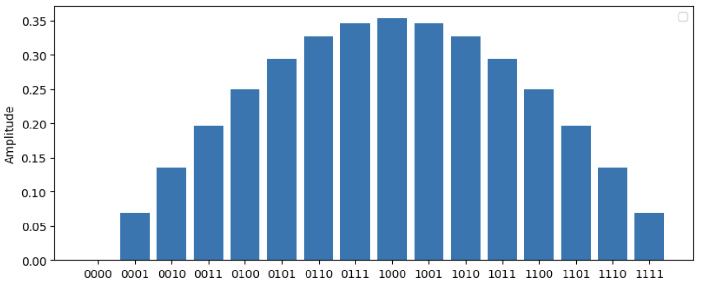
CosineWindowhas been added to prepare an initial state based on a cosine wave function. (#4683)As outlined in 2110.09590, the cosine tapering window is part of a modification to quantum phase estimation that can provide a cubic improvement to the algorithm’s error rate. Using
CosineWindowwill prepare a state whose amplitudes follow a cosinusoidal distribution over the computational basis.import matplotlib.pyplot as plt dev = qml.device('default.qubit', wires=4) @qml.qnode(dev) def example_circuit(): qml.CosineWindow(wires=range(4)) return qml.state() output = example_circuit() plt.style.use("pennylane.drawer.plot") plt.bar(range(len(output)), output) plt.show()
Controlled gate sequences raised to decreasing powers, a sub-block in quantum phase estimation, can now be created with the new
ControlledSequenceoperator. (#4707)To use
ControlledSequence, specify the controlled unitary operator and the control wires,control:dev = qml.device("default.qubit", wires = 4) @qml.qnode(dev) def circuit(): for i in range(3): qml.Hadamard(wires = i) qml.ControlledSequence(qml.RX(0.25, wires = 3), control = [0, 1, 2]) qml.adjoint(qml.QFT)(wires = range(3)) return qml.probs(wires = range(3))
>>> print(circuit())
[0.92059345 0.02637178 0.00729619 0.00423258 0.00360545 0.00423258 0.00729619 0.02637178]
New device capabilities, integration with Catalyst, and more! ⚗️
default.qubitnow uses the newqml.devices.DeviceAPI and functionality inqml.devices.qubit. If you experience any issues with the updateddefault.qubit, please let us know by posting an issue. The old version of the device is still accessible by the short namedefault.qubit.legacy, or directly viaqml.devices.DefaultQubitLegacy. (#4594) (#4436) (#4620) (#4632)This changeover has a number of benefits for
default.qubit, including:The number of wires is now optional — simply having
qml.device("default.qubit")is valid! If wires are not provided at instantiation, the device automatically infers the required number of wires for each circuit provided for execution.dev = qml.device("default.qubit") @qml.qnode(dev) def circuit(): qml.PauliZ(0) qml.RZ(0.1, wires=1) qml.Hadamard(2) return qml.state()
>>> print(qml.draw(circuit)())
0: ──Z────────┤  State
1: ──RZ(0.10)─┤  State
2: ──H────────┤  State
default.qubitis no longer silently swapped out with an interface-appropriate device when the backpropagation differentiation method is used. For example, consider:import jax dev = qml.device("default.qubit", wires=1) @qml.qnode(dev, diff_method="backprop") def f(x): qml.RX(x, wires=0) return qml.expval(qml.PauliZ(0)) f(jax.numpy.array(0.2))
In previous versions of PennyLane, the device will be swapped for the JAX equivalent:
>>> f.device
<DefaultQubitJax device (wires=1, shots=None) at 0x7f8c8bff50a0>
>>> f.device == dev
False
Now,
default.qubitcan itself dispatch to all the interfaces in a backprop-compatible way and hence does not need to be swapped:>>> f.device <default.qubit device (wires=1) at 0x7f20d043b040> >>> f.device == dev True
A QNode that has been decorated with
qjitfrom PennyLane’s Catalyst library for just-in-time hybrid compilation is now compatible withqml.draw. (#4609)import catalyst @catalyst.qjit @qml.qnode(qml.device("lightning.qubit", wires=3)) def circuit(x, y, z, c): """A quantum circuit on three wires.""" @catalyst.for_loop(0, c, 1) def loop(i): qml.Hadamard(wires=i) qml.RX(x, wires=0) loop() qml.RY(y, wires=1) qml.RZ(z, wires=2) return qml.expval(qml.PauliZ(0)) draw = qml.draw(circuit, decimals=None)(1.234, 2.345, 3.456, 1)
>>> print(draw)
0: ──RX──H──┤  <Z>
1: ──H───RY─┤
2: ──RZ─────┤
Improvements 🛠
More PyTrees!
MeasurementProcessandQuantumScriptobjects are now registered as JAX PyTrees. (#4607) (#4608)It is now possible to JIT-compile functions with arguments that are a
MeasurementProcessor aQuantumScript:import jax tape0 = qml.tape.QuantumTape([qml.RX(1.0, 0), qml.RY(0.5, 0)], [qml.expval(qml.PauliZ(0))]) dev = qml.device('lightning.qubit', wires=5) execute_kwargs = {"device": dev, "gradient_fn": qml.gradients.param_shift, "interface":"jax"} jitted_execute = jax.jit(qml.execute, static_argnames=execute_kwargs.keys()) jitted_execute((tape0, ), **execute_kwargs)
Improving QChem and existing algorithms
Computationally expensive functions in
integrals.py,electron_repulsionand_hermite_coulomb, have been modified to replace indexing with slicing for better compatibility with JAX. (#4685)qml.qchem.import_statehas been extended to import more quantum chemistry wavefunctions, from MPS, DMRG and SHCI classical calculations performed with the Block2 and Dice libraries. #4523 #4524 #4626 #4634Check out our how-to guide to learn more about how PennyLane integrates with your favourite quantum chemistry libraries.
The qchem
fermionic_dipoleandparticle_numberfunctions have been updated to use aFermiSentence. The deprecated features for using tuples to represent fermionic operations are removed. (#4546) (#4556)The tensor-network template
qml.MPSnow supports changing theoffsetbetween subsequent blocks for more flexibility. (#4531)Builtin types support with
qml.pauli_decomposehave been improved. (#4577)AmplitudeEmbeddingnow inherits fromStatePrep, allowing for it to not be decomposed when at the beginning of a circuit, thus behaving likeStatePrep. (#4583)qml.cut_circuitis now compatible with circuits that compute the expectation values of Hamiltonians with two or more terms. (#4642)
Next-generation device API
default.qubitnow tracks the number of equivalent qpu executions and total shots when the device is sampling. Note that"simulations"denotes the number of simulation passes, whereas"executions"denotes how many different computational bases need to be sampled in. Additionally, the newdefault.qubittracks the results ofdevice.execute. (#4628) (#4649)DefaultQubitcan now accept ajax.random.PRNGKeyas aseedto set the key for the JAX pseudo random number generator when using the JAX interface. This corresponds to theprng_keyondefault.qubit.jaxin the old API. (#4596)The
JacobianProductCalculatorabstract base class and implementationsTransformJacobianProductsDeviceDerivatives, andDeviceJacobianProductshave been added topennylane.interfaces.jacobian_products. (#4435) (#4527) (#4637)DefaultQubitdispatches to a faster implementation for applyingParametrizedEvolutionto a state when it is more efficient to evolve the state than the operation matrix. (#4598) (#4620)Wires can be provided to the new device API. (#4538) (#4562)
qml.sample()in the new device API now returns anp.int64array instead ofnp.bool8. (#4539)The new device API now has a
repr()method. (#4562)DefaultQubitnow works as expected with measurement processes that don’t specify wires. (#4580)Various improvements to measurements have been made for feature parity between
default.qubit.legacyand the newDefaultQubit. This includes not trying to squeeze batchedCountsMPresults and implementingMutualInfoMP.map_wires. (#4574)devices.qubit.simulatenow accepts an interface keyword argument. If a QNode withDefaultQubitspecifies an interface, the result will be computed with that interface. (#4582)ShotAdaptiveOptimizerhas been updated to pass shots to QNode executions instead of overriding device shots before execution. This makes it compatible with the new device API. (#4599)pennylane.devices.preprocessnow offers the transformsdecompose,validate_observables,validate_measurements,validate_device_wires,validate_multiprocessing_workers,warn_about_trainable_observables, andno_samplingto assist in constructing devices under the new device API. (#4659)Updated
qml.device,devices.preprocessingand thetape_expand.set_decompositioncontext manager to bringDefaultQubitto feature parity withdefault.qubit.legacywith regards to using custom decompositions. TheDefaultQubitdevice can now be included in aset_decompositioncontext or initialized with acustom_decompsdictionary, as well as a custommax_depthfor decomposition. (#4675)
Other improvements
The
StateMPmeasurement now accepts a wire order (e.g., a device wire order). Theprocess_statemethod will re-order the given state to go from the inputted wire-order to the process’s wire-order. If the process’s wire-order contains extra wires, it will assume those are in the zero-state. (#4570) (#4602)Methods called
add_transformandinsert_front_transformhave been added toTransformProgram. (#4559)Instances of the
TransformProgramclass can now be added together. (#4549)Transforms can now be applied to devices following the new device API. (#4667)
All gradient transforms have been updated to the new transform program system. (#4595)
Multi-controlled operations with a single-qubit special unitary target can now automatically decompose. (#4697)
pennylane.defer_measurementswill now exit early if the input does not contain mid circuit measurements. (#4659)The density matrix aspects of
StateMPhave been split into their own measurement process calledDensityMatrixMP. (#4558)StateMeasurement.process_statenow assumes that the input is flat.ProbabilityMP.process_statehas been updated to reflect this assumption and avoid redundant reshaping. (#4602)qml.expreturns a more informative error message when decomposition is unavailable for non-unitary operators. (#4571)Added
qml.math.get_deep_interfaceto get the interface of a scalar hidden deep in lists or tuples. (#4603)Updated
qml.math.ndimandqml.math.shapeto work with built-in lists or tuples that contain interface-specific scalar dat (e.g.,[(tf.Variable(1.1), tf.Variable(2.2))]). (#4603)When decomposing a unitary matrix with
one_qubit_decompositionand opting to include theGlobalPhasein the decomposition, the phase is no longer cast todtype=complex. (#4653)_qfunc_outputhas been removed fromQuantumScript, as it is no longer necessary. There is still a_qfunc_outputproperty onQNodeinstances. (#4651)qml.data.loadproperly handles parameters that come after'full'(#4663)The
qml.jordan_wignerfunction has been modified to optionally remove the imaginary components of the computed qubit operator, if imaginary components are smaller than a threshold. (#4639)qml.data.loadcorrectly performs a full download of the dataset after a partial download of the same dataset has already been performed. (#4681)The performance of
qml.data.load()has been improved when partially loading a dataset (#4674)Plots generated with the
pennylane.drawer.plotstyle ofmatplotlib.pyplotnow have black axis labels and are generated at a default DPI of 300. (#4690)Shallow copies of the
QNodenow also copy theexecute_kwargsand transform program. When applying a transform to aQNode, the new qnode is only a shallow copy of the original and thus keeps the same device. (#4736)QubitDeviceandCountsMPare updated to disregard samples containing failed hardware measurements (record asnp.NaN) when tallying samples, rather than counting failed measurements as ground-state measurements, and to displayqml.countscoming from these hardware devices correctly. (#4739)
Breaking changes 💔
qml.defer_measurementsnow raises an error if a transformed circuit measuresqml.probs,qml.sample, orqml.countswithout any wires or observable, or if it measuresqml.state. (#4701)The device test suite now converts device keyword arguments to integers or floats if possible. (#4640)
MeasurementProcess.eigvals()now raises anEigvalsUndefinedErrorif the measurement observable does not have eigenvalues. (#4544)The
__eq__and__hash__methods ofOperatorandMeasurementProcessno longer rely on the object’s address in memory. Using==with operators and measurement processes will now behave the same asqml.equal, and objects of the same type with the same data and hyperparameters will have the same hash. (#4536)In the following scenario, the second and third code blocks show the previous and current behaviour of operator and measurement process equality, determined by
==:op1 = qml.PauliX(0) op2 = qml.PauliX(0) op3 = op1
Old behaviour:
>>> op1 == op2
False
>>> op1 == op3
True
New behaviour:
>>> op1 == op2
True
>>> op1 == op3
True
The
__hash__dunder method defines the hash of an object. The default hash of an object is determined by the objects memory address. However, the new hash is determined by the properties and attributes of operators and measurement processes. Consider the scenario below. The second and third code blocks show the previous and current behaviour.op1 = qml.PauliX(0) op2 = qml.PauliX(0)
Old behaviour:
>>> print({op1, op2})
{PauliX(wires=[0]), PauliX(wires=[0])}
New behaviour:
>>> print({op1, op2})
{PauliX(wires=[0])}
The old return type and associated functions
qml.enable_returnandqml.disable_returnhave been removed. (#4503)The
modekeyword argument inQNodehas been removed. Please usegrad_on_executioninstead. (#4503)The CV observables
qml.Xandqml.Phave been removed. Please useqml.QuadXandqml.QuadPinstead. (#4533)The
sampler_seedargument ofqml.gradients.spsa_gradhas been removed. Instead, thesampler_rngargument should be set, either to an integer value, which will be used to create a PRNG internally, or to a NumPy pseudo-random number generator (PRNG) created vianp.random.default_rng(seed). (#4550)The
QuantumScript.set_parametersmethod and theQuantumScript.datasetter have been removed. Please useQuantumScript.bind_new_parametersinstead. (#4548)The method
tape.unwrap()and correspondingUnwrapTapeandUnwrapclasses have been removed. Instead oftape.unwrap(), useqml.transforms.convert_to_numpy_parameters. (#4535)The
RandomLayers.compute_decompositionkeyword argumentratio_imprivitivehas been changed toratio_imprimto match the call signature of the operation. (#4552)The private
TmpPauliRotoperator used forSpecialUnitaryno longer decomposes to nothing when the theta value is trainable. (#4585)ProbabilityMP.marginal_probhas been removed. Its contents have been moved intoprocess_state, which effectively just calledmarginal_probwithnp.abs(state) ** 2. (#4602)
Deprecations 👋
The following decorator syntax for transforms has been deprecated and will raise a warning: (#4457)
@transform_fn(**transform_kwargs)
@qml.qnode(dev)
def circuit():
    ...
If you are using a transform that has supporting
transform_kwargs, please call the transform directly usingcircuit = transform_fn(circuit, **transform_kwargs), or usefunctools.partial:@functools.partial(transform_fn, **transform_kwargs) @qml.qnode(dev) def circuit(): ...
The
prepkeyword argument inQuantumScripthas been deprecated and will be removed fromQuantumScript.StatePrepBaseoperations should be placed at the beginning of theopslist instead. (#4554)qml.gradients.pulse_generatorhas been renamed toqml.gradients.pulse_odegento adhere to paper naming conventions. During v0.33,pulse_generatoris still available but raises a warning. (#4633)
Documentation 📝
A warning section in the docstring for
DefaultQubitregarding the start method used in multiprocessing has been added. This may help users circumvent issues arising in Jupyter notebooks on macOS for example. (#4622)Documentation improvements to the new device API have been made. The documentation now correctly states that interface-specific parameters are only passed to the device for backpropagation derivatives. (#4542)
Functions for qubit-simulation to the
qml.devicessub-page of the “Internal” section have been added. Note that these functions are unstable while device upgrades are underway. (#4555)A documentation improvement to the usage example in the
qml.QuantumMonteCarlopage has been made. An integral was missing the differential \(dx\). (#4593)A documentation improvement for the use of the
pennylanestyle ofqml.drawerand thepennylane.drawer.plotstyle ofmatplotlib.pyplothas been made by clarifying the use of the default font. (#4690)
Bug fixes 🐛
Jax jit now works when a probability measurement is broadcasted onto all wires. (#4742)
Fixed
LocalHilbertSchmidt.compute_decompositionso that the template can be used in a QNode. (#4719)Fixes
transforms.transpilewith arbitrary measurement processes. (#4732)Providing
work_wires=Nonetoqml.GroverOperatorno longer interpretsNoneas a wire. (#4668)Fixed an issue where the
__copy__method of theqml.Select()operator attempted to access un-initialized data. (#4551)Fixed the
skip_firstoption inexpand_tape_state_prep. (#4564)convert_to_numpy_parametersnow usesqml.ops.functions.bind_new_parameters. This reinitializes the operation and makes sure everything references the new NumPy parameters. (#4540)tf.functionno longer breaksProbabilityMP.process_state, which is needed by new devices. (#4470)Fixed unit tests for
qml.qchem.mol_data. (#4591)Fixed
ProbabilityMP.process_stateso that it allows for proper Autograph compilation. Without this, decorating a QNode that returns anexpvalwithtf.functionwould fail when computing the expectation. (#4590)The
torch.nn.Moduleproperties are now accessible on apennylane.qnn.TorchLayer. (#4611)qml.math.takewith Pytorch now returnstensor[..., indices]when the user requests the last axis (axis=-1). Without the fix, it would wrongly returntensor[indices]. (#4605)Ensured the logging
TRACElevel works with gradient-free execution. (#4669)
Contributors ✍️
This release contains contributions from (in alphabetical order):
Guillermo Alonso, Utkarsh Azad, Thomas Bromley, Isaac De Vlugt, Jack Brown, Stepan Fomichev, Joana Fraxanet, Diego Guala, Soran Jahangiri, Edward Jiang, Korbinian Kottmann, Ivana Kurečić Christina Lee, Lillian M. A. Frederiksen, Vincent Michaud-Rioux, Romain Moyard, Daniel F. Nino, Lee James O’Riordan, Mudit Pandey, Matthew Silverman, Jay Soni.
- orphan
Release 0.32.0¶
New features since last release
Encode matrices using a linear combination of unitaries ⛓️️
It is now possible to encode an operator
Ainto a quantum circuit by decomposing it into a linear combination of unitaries using PREP (qml.StatePrep) and SELECT (qml.Select) routines. (#4431) (#4437) (#4444) (#4450) (#4506) (#4526)Consider an operator
Acomposed of a linear combination of Pauli terms:>>> A = qml.PauliX(2) + 2 * qml.PauliY(2) + 3 * qml.PauliZ(2)
A decomposable block-encoding circuit can be created:
def block_encode(A, control_wires):
    probs = A.coeffs / np.sum(A.coeffs)
    state = np.pad(np.sqrt(probs, dtype=complex), (0, 1))
    unitaries = A.ops

    qml.StatePrep(state, wires=control_wires)
    qml.Select(unitaries, control=control_wires)
    qml.adjoint(qml.StatePrep)(state, wires=control_wires)
>>> print(qml.draw(block_encode, show_matrices=False)(A, control_wires=[0, 1]))
0: ─╭|Ψ⟩─╭Select─╭|Ψ⟩†─┤
1: ─╰|Ψ⟩─├Select─╰|Ψ⟩†─┤
2: ──────╰Select───────┤
This circuit can be used as a building block within a larger QNode to perform algorithms such as QSVT and Hamiltonian simulation.
Decomposing a Hermitian matrix into a linear combination of Pauli words via
qml.pauli_decomposeis now faster and differentiable. (#4395) (#4479) (#4493)def find_coeffs(p): mat = np.array([[3, p], [p, 3]]) A = qml.pauli_decompose(mat) return A.coeffs
>>> import jax
>>> from jax import numpy as np
>>> jax.jacobian(find_coeffs)(np.array(2.))
Array([0., 1.], dtype=float32, weak_type=True)
Monitor PennyLane's inner workings with logging 📃
Python-native logging can now be enabled with
qml.logging.enable_logging(). (#4377) (#4383)Consider the following code that is contained in
my_code.py:import pennylane as qml qml.logging.enable_logging() # enables logging dev = qml.device("default.qubit", wires=2) @qml.qnode(dev) def f(x): qml.RX(x, wires=0) return qml.state() f(0.5)
Executing
my_code.pywith logging enabled will detail every step in PennyLane’s pipeline that gets used to run your code.$ python my_code.py [1967-02-13 15:18:38,591][DEBUG][<PID 8881:MainProcess>] - pennylane.qnode.__init__()::"Creating QNode(func=<function f at 0x7faf2a6fbaf0>, device=<DefaultQubit device (wires=2, shots=None) at 0x7faf2a689b50>, interface=auto, diff_method=best, expansion_strategy=gradient, max_expansion=10, grad_on_execution=best, mode=None, cache=True, cachesize=10000, max_diff=1, gradient_kwargs={}" ...Additional logging configuration settings can be specified by modifying the contents of the logging configuration file, which can be located by running
qml.logging.config_path(). Follow our logging docs page for more details!
More input states for quantum chemistry calculations ⚛️
Input states obtained from advanced quantum chemistry calculations can be used in a circuit. (#4427) (#4433) (#4461) (#4476) (#4505)
Quantum chemistry calculations rely on an initial state that is typically selected to be the trivial Hartree-Fock state. For molecules with a complicated electronic structure, using initial states obtained from affordable post-Hartree-Fock calculations helps to improve the efficiency of the quantum simulations. These calculations can be done with external quantum chemistry libraries such as PySCF.
It is now possible to import a PySCF solver object in PennyLane and extract the corresponding wave function in the form of a state vector that can be directly used in a circuit. First, perform your classical quantum chemistry calculations and then use the qml.qchem.import_state function to import the solver object and return a state vector.
   >>> from pyscf import gto, scf, ci
   >>> mol = gto.M(atom=[['H', (0, 0, 0)], ['H', (0,0,0.71)]], basis='sto6g')
   >>> myhf = scf.UHF(mol).run()
   >>> myci = ci.UCISD(myhf).run()
   >>> wf_cisd = qml.qchem.import_state(myci, tol=1e-1)
   >>> print(wf_cisd)
   [ 0.        +0.j  0.        +0.j  0.        +0.j  0.1066467 +0.j
     1.        +0.j  0.        +0.j  0.        +0.j  0.        +0.j
     2.        +0.j  0.        +0.j  0.        +0.j  0.        +0.j
    -0.99429698+0.j  0.        +0.j  0.        +0.j  0.        +0.j]

The state vector can be implemented in a circuit using ``qml.StatePrep``.
   >>> dev = qml.device('default.qubit', wires=4)
   >>> @qml.qnode(dev)
   ... def circuit():
   ...     qml.StatePrep(wf_cisd, wires=range(4))
   ...     return qml.state()
   >>> print(circuit())
   [ 0.        +0.j  0.        +0.j  0.        +0.j  0.1066467 +0.j
     1.        +0.j  0.        +0.j  0.        +0.j  0.        +0.j
     2.        +0.j  0.        +0.j  0.        +0.j  0.        +0.j
    -0.99429698+0.j  0.        +0.j  0.        +0.j  0.        +0.j]

The currently supported post-Hartree-Fock methods are RCISD, UCISD, RCCSD, and UCCSD which
denote restricted (R) and unrestricted (U) configuration interaction (CI) and coupled cluster (CC)
calculations with single and double (SD) excitations.
Reuse and reset qubits after mid-circuit measurements ♻️
PennyLane now allows you to define circuits that reuse a qubit after a mid-circuit measurement has taken place. Optionally, the wire can also be reset to the \(|0\rangle\) state. (#4402) (#4432)
Post-measurement reset can be activated by setting
reset=Truewhen calling qml.measure. In this version of PennyLane, executing circuits with qubit reuse will result in the defer_measurements transform being applied. This transform replaces each reused wire with an additional qubit. However, future releases of PennyLane will explore device-level support for qubit reuse without consuming additional qubits.Qubit reuse and reset is also fully differentiable:
dev = qml.device("default.qubit", wires=4)

@qml.qnode(dev)
def circuit(p):
    qml.RX(p, wires=0)
    m = qml.measure(0, reset=True)
    qml.cond(m, qml.Hadamard)(1)

    qml.RX(p, wires=0)
    m = qml.measure(0)
    qml.cond(m, qml.Hadamard)(1)
    return qml.expval(qml.PauliZ(1))
>>> jax.grad(circuit)(0.4)
Array(-0.35867804, dtype=float32, weak_type=True)
You can read more about mid-circuit measurements in the documentation, and stay tuned for more mid-circuit measurement features in the next few releases!
Improvements 🛠
A new PennyLane drawing style
Circuit drawings and plots can now be created following a PennyLane style. (#3950)
The
qml.draw_mplfunction accepts astyle='pennylane'argument to create PennyLane themed circuit diagrams:def circuit(x, z): qml.QFT(wires=(0,1,2,3)) qml.Toffoli(wires=(0,1,2)) qml.CSWAP(wires=(0,2,3)) qml.RX(x, wires=0) qml.CRZ(z, wires=(3,0)) return qml.expval(qml.PauliZ(0)) qml.draw_mpl(circuit, style="pennylane")(1, 1)
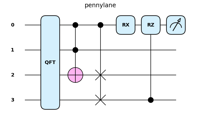
PennyLane-styled plots can also be drawn by passing
"pennylane.drawer.plot"to Matplotlib’splt.style.usefunction:import matplotlib.pyplot as plt plt.style.use("pennylane.drawer.plot") for i in range(3): plt.plot(np.random.rand(10))
If the font Quicksand Bold isn’t available, an available default font is used instead.
Making operators immutable and PyTrees
Any class inheriting from
Operatoris now automatically registered as a pytree with JAX. This unlocks the ability to jit functions ofOperator. (#4458)>>> op = qml.adjoint(qml.RX(1.0, wires=0)) >>> jax.jit(qml.matrix)(op) Array([[0.87758255-0.j , 0. +0.47942555j], [0. +0.47942555j, 0.87758255-0.j ]], dtype=complex64, weak_type=True) >>> jax.tree_util.tree_map(lambda x: x+1, op) Adjoint(RX(2.0, wires=[0]))
All
Operatorobjects now defineOperator._flattenandOperator._unflattenmethods that separate trainable from untrainable components. These methods will be used in serialization and pytree registration. Custom operations may need an update to ensure compatibility with new PennyLane features. (#4483) (#4314)The
QuantumScriptclass now has abind_new_parametersmethod that allows creation of newQuantumScriptobjects with the provided parameters. (#4345)The
qml.gradientsmodule no longer mutates operators in-place for any gradient transforms. Instead, operators that need to be mutated are copied with new parameters. (#4220)PennyLane no longer directly relies on
Operator.__eq__. (#4398)qml.equalno longer raises errors when operators or measurements of different types are compared. Instead, it returnsFalse. (#4315)
Transforms
Transform programs are now integrated with the QNode. (#4404)
def null_postprocessing(results: qml.typing.ResultBatch) -> qml.typing.Result:
    return results[0]

@qml.transforms.core.transform
def scale_shots(tape: qml.tape.QuantumTape, shot_scaling) -> (Tuple[qml.tape.QuantumTape], Callable):
    new_shots = tape.shots.total_shots * shot_scaling
    new_tape = qml.tape.QuantumScript(tape.operations, tape.measurements, shots=new_shots)
    return (new_tape, ), null_postprocessing

dev = qml.devices.experimental.DefaultQubit2()

@partial(scale_shots, shot_scaling=2)
@qml.qnode(dev, interface=None)
def circuit():
    return qml.sample(wires=0)
>>> circuit(shots=1)
array([False, False])
Transform Programs,
qml.transforms.core.TransformProgram, can now be called on a batch of circuits and return a new batch of circuits and a single post processing function. (#4364)TransformDispatchernow allows registration of custom QNode transforms. (#4466)QNode transforms in
qml.qinfonow support custom wire labels. #4331qml.transforms.adjoint_metric_tensornow uses the simulation tools inqml.devices.qubitinstead of private methods ofqml.devices.DefaultQubit. (#4456)Auxiliary wires and device wires are now treated the same way in
qml.transforms.metric_tensoras inqml.gradients.hadamard_grad. All valid wire input formats foraux_wireare supported. (#4328)
Next-generation device API
The experimental device interface has been integrated with the QNode for JAX, JAX-JIT, TensorFlow and PyTorch. (#4323) (#4352) (#4392) (#4393)
The experimental
DefaultQubit2device now supports computing VJPs and JVPs using the adjoint method. (#4374)New functions called
adjoint_jvpandadjoint_vjpthat compute the JVP and VJP of a tape using the adjoint method have been added toqml.devices.qubit.adjoint_jacobian(#4358)DefaultQubit2now accepts amax_workersargument which controls multiprocessing. AProcessPoolExecutorexecutes tapes asynchronously using a pool of at mostmax_workersprocesses. Ifmax_workersisNoneor not given, only the current process executes tapes. If you experience any issue, say using JAX, TensorFlow, Torch, try settingmax_workerstoNone. (#4319) (#4425)qml.devices.experimental.Devicenow accepts a shots keyword argument and has ashotsproperty. This property is only used to set defaults for a workflow, and does not directly influence the number of shots used in executions or derivatives. (#4388)expand_fn()forDefaultQubit2has been updated to decomposeStatePrepoperations present in the middle of a circuit. (#4444)If no seed is specified on initialization with
DefaultQubit2, the local random number generator will be seeded from NumPy’s global random number generator. (#4394)
Improvements to machine learning library interfaces
pennylane/interfaceshas been refactored. Theexecute_fnpassed to the machine learning framework boundaries is now responsible for converting parameters to NumPy. The gradients module can now handle TensorFlow parameters, but gradient tapes now retain the originaldtypeinstead of converting tofloat64. This may cause instability with finite-difference differentiation andfloat32parameters. The machine learning boundary functions are now uncoupled from their legacy counterparts. (#4415)qml.interfaces.set_shotsnow accepts aShotsobject as well asint‘s and tuples ofint‘s. (#4388)Readability improvements and stylistic changes have been made to
pennylane/interfaces/jax_jit_tuple.py(#4379)
Pulses
A
HardwareHamiltoniancan now be summed withintorfloatobjects. A sequence ofHardwareHamiltonians can now be summed via the builtinsum. (#4343)qml.pulse.transmon_drivehas been updated in accordance with 1904.06560. In particular, the functional form has been changed from \(\Omega(t)(\cos(\omega_d t + \phi) X - \sin(\omega_d t + \phi) Y)$ to $\Omega(t) \sin(\omega_d t + \phi) Y\). (#4418) (#4465) (#4478) (#4418)
Other improvements
The
qchemmodule has been upgraded to use the fermionic operators of thefermimodule. #4336 #4521The calculation of
Sum,Prod,SProd,PauliWord, andPauliSentencesparse matrices are orders of magnitude faster. (#4475) (#4272) (#4411)A function called
qml.math.fidelity_statevectorthat computes the fidelity between two state vectors has been added. (#4322)qml.ctrl(qml.PauliX)returns aCNOT,Toffoli, orMultiControlledXoperation instead ofControlled(PauliX). (#4339)When given a callable,
qml.ctrlnow does its custom pre-processing on all queued operators from the callable. (#4370)The
qchemfunctionsprimitive_normandcontracted_normhave been modified to be compatible with higher versions of SciPy. The private function_fac2for computing double factorials has also been added. #4321tape_expandnow usesOperator.decompositioninstead ofOperator.expandin order to make more performant choices. (#4355)CI now runs tests with TensorFlow 2.13.0 (#4472)
All tests in CI and pre-commit hooks now enable linting. (#4335)
The default label for a
StatePrepBaseoperator is now|Ψ⟩. (#4340)Device.default_expand_fn()has been updated to decomposeqml.StatePrepoperations present in the middle of a provided circuit. (#4437)QNode.constructhas been updated to only apply theqml.defer_measurementstransform if the device does not natively support mid-circuit measurements. (#4516)The application of the
qml.defer_measurementstransform has been moved fromQNode.constructtoqml.Device.batch_transformto allow more fine-grain control over whendefer_measurementsshould be used. (#4432)The label for
ParametrizedEvolutioncan display parameters with the requested format as set by the kwargdecimals. Array-like parameters are displayed in the same format as matrices and stored in the cache. (#4151)
Breaking changes 💔
Applying gradient transforms to broadcasted/batched tapes has been deactivated until it is consistently supported for QNodes as well. (#4480)
Gradient transforms no longer implicitly cast
float32parameters tofloat64. Finite difference differentiation withfloat32parameters may no longer give accurate results. (#4415)The
do_queuekeyword argument inqml.operation.Operatorhas been removed. Instead of settingdo_queue=False, use theqml.QueuingManager.stop_recording()context. (#4317)Operator.expandnow uses the output ofOperator.decompositioninstead of what it queues. (#4355)The gradients module no longer needs shot information passed to it explicitly, as the shots are on the tapes. (#4448)
qml.StatePrephas been renamed toqml.StatePrepBaseandqml.QubitStateVectorhas been renamed toqml.StatePrep.qml.operation.StatePrepandqml.QubitStateVectorare still accessible. (#4450)Support for Python 3.8 has been dropped. (#4453)
MeasurementValue‘s signature has been updated to accept a list ofMidMeasureMP‘s rather than a list of their IDs. (#4446)The
grouping_typeandgrouping_methodkeyword arguments have been removed fromqchem.molecular_hamiltonian. (#4301)zyz_decompositionandxyx_decompositionhave been removed. Useone_qubit_decompositioninstead. (#4301)LieAlgebraOptimizerhas been removed. UseRiemannianGradientOptimizerinstead. (#4301)Operation.base_namehas been removed. (#4301)QuantumScript.namehas been removed. (#4301)qml.math.reduced_dmhas been removed. Useqml.math.reduce_dmorqml.math.reduce_statevectorinstead. (#4301)The
qml.specsdictionary no longer supports direct key access to certain keys. (#4301)Instead, these quantities can be accessed as fields of the new
Resourcesobject saved underspecs_dict["resources"]:num_operationsis no longer supported, usespecs_dict["resources"].num_gatesnum_used_wiresis no longer supported, usespecs_dict["resources"].num_wiresgate_typesis no longer supported, usespecs_dict["resources"].gate_typesgate_sizesis no longer supported, usespecs_dict["resources"].gate_sizesdepthis no longer supported, usespecs_dict["resources"].depth
qml.math.purity,qml.math.vn_entropy,qml.math.mutual_info,qml.math.fidelity,qml.math.relative_entropy, andqml.math.max_entropyno longer support state vectors as input. (#4322)The private
QuantumScript._preplist has been removed, and prep operations now go into the_opslist. (#4485)
Deprecations 👋
qml.enable_returnandqml.disable_returnhave been deprecated. Please avoid callingdisable_return, as the old return system has been deprecated along with these switch functions. (#4316)qml.qchem.jordan_wignerhas been deprecated. Useqml.jordan_wignerinstead. List input to define the fermionic operator has also been deprecated; the fermionic operators in theqml.fermimodule should be used instead. (#4332)The
qml.RandomLayers.compute_decompositionkeyword argumentratio_imprimitivewill be changed toratio_imprimto match the call signature of the operation. (#4314)The CV observables
qml.Xandqml.Phave been deprecated. Useqml.QuadXandqml.QuadPinstead. (#4330)The method
tape.unwrap()and correspondingUnwrapTapeandUnwrapclasses have been deprecated. Useconvert_to_numpy_parametersinstead. (#4344)The
modekeyword argument in QNode has been deprecated, as it was only used in the old return system (which has also been deprecated). Please usegrad_on_executioninstead. (#4316)The
QuantumScript.set_parametersmethod and theQuantumScript.datasetter have been deprecated. Please useQuantumScript.bind_new_parametersinstead. (#4346)The
__eq__and__hash__dunder methods ofOperatorandMeasurementProcesswill now raise warnings to reflect upcoming changes to operator and measurement process equality and hashing. (#4144) (#4454) (#4489) (#4498)The
sampler_seedargument ofqml.gradients.spsa_gradhas been deprecated, along with a bug fix of the seed-setting behaviour. Instead, thesampler_rngargument should be set, either to an integer value, which will be used to create a PRNG internally or to a NumPy pseudo-random number generator created vianp.random.default_rng(seed). (4165)
Documentation 📝
The
qml.pulse.transmon_interactionandqml.pulse.transmon_drivedocumentation has been updated. #4327qml.ApproxTimeEvolution.compute_decomposition()now has a code example. (#4354)The documentation for
qml.devices.experimental.Devicehas been improved to clarify some aspects of its use. (#4391)Input types and sources for operators in
qml.import_operatorare specified. (#4476)
Bug fixes 🐛
qml.Projectoris pickle-able again. (#4452)_copy_and_shift_paramsdoes not cast or convert integral types, just relying on+and*‘s casting rules in this case. (#4477)Sparse matrix calculations of
SProds containing aTensorare now allowed. When usingTensor.sparse_matrix(), it is recommended to use thewire_orderkeyword argument overwires. (#4424)op.adjointhas been replaced withqml.adjointinQNSPSAOptimizer. (#4421)jax.ad(deprecated) has been replaced byjax.interpreters.ad. (#4403)metric_tensorstops accidentally catching errors that stem from flawed wires assignments in the original circuit, leading to recursion errors. (#4328)A warning is now raised if control indicators are hidden when calling
qml.draw_mpl(#4295)qml.qinfo.puritynow produces correct results with custom wire labels. (#4331)default.qutritnow supports all qutrit operations used withqml.adjoint. (#4348)The observable data of
qml.GellMannnow includes its index, allowing correct comparison between instances ofqml.GellMann, as well as Hamiltonians and Tensors containingqml.GellMann. (#4366)qml.transforms.merge_amplitude_embeddingnow works correctly when theAmplitudeEmbeddings have a batch dimension. (#4353)The
jordan_wignerfunction has been modified to work with Hamiltonians built with an active space. (#4372)When a
styleoption is not provided,qml.draw_mpluses the current style set fromqml.drawer.use_styleinstead ofblack_white. (#4357)qml.devices.qubit.preprocess.validate_and_expand_adjointno longer sets the trainable parameters of the expanded tape. (#4365)qml.default_expand_fnnow selectively expands operations or measurements allowing more operations to be executed in circuits when measuring non-qwc Hamiltonians. (#4401)qml.ControlledQubitUnitaryno longer reportshas_decompositionasTruewhen it does not really have a decomposition. (#4407)qml.transforms.split_non_commutingnow correctly works on tapes containing bothexpvalandvarmeasurements. (#4426)Subtracting a
Prodfrom another operator now works as expected. (#4441)The
sampler_seedargument ofqml.gradients.spsa_gradhas been changed tosampler_rng. One can either provide an integer, which will be used to create a PRNG internally. Previously, this lead to the same direction being sampled, whennum_directionsis greater than 1. Alternatively, one can provide a NumPy PRNG, which allows reproducibly callingspsa_gradwithout getting the same results every time. (4165) (4482)qml.math.get_dtype_namenow works with autograd array boxes. (#4494)The backprop gradient of
qml.math.fidelityis now correct. (#4380)
Contributors ✍️
This release contains contributions from (in alphabetical order):
Utkarsh Azad, Thomas Bromley, Isaac De Vlugt, Amintor Dusko, Stepan Fomichev, Lillian M. A. Frederiksen, Soran Jahangiri, Edward Jiang, Korbinian Kottmann, Ivana Kurečić, Christina Lee, Vincent Michaud-Rioux, Romain Moyard, Lee James O’Riordan, Mudit Pandey, Borja Requena, Matthew Silverman, Jay Soni, David Wierichs, Frederik Wilde.
- orphan
Release 0.31.0¶
New features since last release
Seamlessly create and combine fermionic operators 🔬
Fermionic operators and arithmetic are now available. (#4191) (#4195) (#4200) (#4201) (#4209) (#4229) (#4253) (#4255) (#4262) (#4278)
There are a couple of ways to create fermionic operators with this new feature:
qml.FermiCandqml.FermiA: the fermionic creation and annihilation operators, respectively. These operators are defined by passing the index of the orbital that the fermionic operator acts on. For instance, the operatorsa⁺(0)anda(3)are respectively constructed as>>> qml.FermiC(0) a⁺(0) >>> qml.FermiA(3) a(3)
These operators can be composed with (
*) and linearly combined with (+and-) other Fermi operators to create arbitrary fermionic Hamiltonians. Multiplying several Fermi operators together creates an operator that we call a Fermi word:>>> word = qml.FermiC(0) * qml.FermiA(0) * qml.FermiC(3) * qml.FermiA(3) >>> word a⁺(0) a(0) a⁺(3) a(3)
Fermi words can be linearly combined to create a fermionic operator that we call a Fermi sentence:
>>> sentence = 1.2 * word - 0.345 * qml.FermiC(3) * qml.FermiA(3)
>>> sentence
1.2 * a⁺(0) a(0) a⁺(3) a(3)
- 0.345 * a⁺(3) a(3)
via qml.fermi.from_string: create a fermionic operator that represents multiple creation and annihilation operators being multiplied by each other (a Fermi word).
>>> qml.fermi.from_string('0+ 1- 0+ 1-')
a⁺(0) a(1) a⁺(0) a(1)
>>> qml.fermi.from_string('0^ 1 0^ 1')
a⁺(0) a(1) a⁺(0) a(1)
Fermi words created with
from_stringcan also be linearly combined to create a Fermi sentence:>>> word1 = qml.fermi.from_string('0+ 0- 3+ 3-') >>> word2 = qml.fermi.from_string('3+ 3-') >>> sentence = 1.2 * word1 + 0.345 * word2 >>> sentence 1.2 * a⁺(0) a(0) a⁺(3) a(3) + 0.345 * a⁺(3) a(3)
Additionally, any fermionic operator, be it a single fermionic creation/annihilation operator, a Fermi word, or a Fermi sentence, can be mapped to the qubit basis by using qml.jordan_wigner:
>>> qml.jordan_wigner(sentence)
((0.4725+0j)*(Identity(wires=[0]))) + ((-0.4725+0j)*(PauliZ(wires=[3]))) + ((-0.3+0j)*(PauliZ(wires=[0]))) + ((0.3+0j)*(PauliZ(wires=[0]) @ PauliZ(wires=[3])))
Learn how to create fermionic Hamiltonians describing some simple chemical systems by checking out our fermionic operators demo!
Workflow-level resource estimation 🧮
PennyLane’s Tracker now monitors the resource requirements of circuits being executed by the device. (#4045) (#4110)
Suppose we have a workflow that involves executing circuits with different qubit numbers. We can obtain the resource requirements as a function of the number of qubits by executing the workflow with the
Trackercontext:dev = qml.device("default.qubit", wires=4) @qml.qnode(dev) def circuit(n_wires): for i in range(n_wires): qml.Hadamard(i) return qml.probs(range(n_wires)) with qml.Tracker(dev) as tracker: for i in range(1, 5): circuit(i)
The resource requirements of individual circuits can then be inspected as follows:
>>> resources = tracker.history["resources"]
>>> resources[0]
wires: 1
gates: 1
depth: 1
shots: Shots(total=None)
gate_types:
{'Hadamard': 1}
gate_sizes:
{1: 1}
>>> [r.num_wires for r in resources]
[1, 2, 3, 4]
Moreover, it is possible to predict the resource requirements without evaluating circuits using the
null.qubitdevice, which follows the standard execution pipeline but returns numeric zeros. Consider the following workflow that takes the gradient of a50-qubit circuit:n_wires = 50 dev = qml.device("null.qubit", wires=n_wires) weight_shape = qml.StronglyEntanglingLayers.shape(2, n_wires) weights = np.random.random(weight_shape, requires_grad=True) @qml.qnode(dev, diff_method="parameter-shift") def circuit(weights): qml.StronglyEntanglingLayers(weights, wires=range(n_wires)) return qml.expval(qml.PauliZ(0)) with qml.Tracker(dev) as tracker: qml.grad(circuit)(weights)
The tracker can be inspected to extract resource requirements without requiring a 50-qubit circuit run:
>>> tracker.totals
{'executions': 451, 'batches': 2, 'batch_len': 451}
>>> tracker.history["resources"][0]
wires: 50
gates: 200
depth: 77
shots: Shots(total=None)
gate_types:
{'Rot': 100, 'CNOT': 100}
gate_sizes:
{1: 100, 2: 100}
Custom operations can now be constructed that solely define resource requirements — an explicit decomposition or matrix representation is not needed. (#4033)
PennyLane is now able to estimate the total resource requirements of circuits that include one or more of these operations, allowing you to estimate requirements for high-level algorithms composed of abstract subroutines.
These operations can be defined by inheriting from ResourcesOperation and overriding the
resources()method to return an appropriate Resources object:class CustomOp(qml.resource.ResourcesOperation): def resources(self): n = len(self.wires) r = qml.resource.Resources( num_wires=n, num_gates=n ** 2, depth=5, ) return r
>>> wires = [0, 1, 2]
>>> c = CustomOp(wires)
>>> c.resources()
wires: 3
gates: 9
depth: 5
shots: Shots(total=None)
gate_types:
{}
gate_sizes:
{}
A quantum circuit that contains
CustomOpcan be created and inspected using qml.specs:dev = qml.device("default.qubit", wires=wires) @qml.qnode(dev) def circ(): qml.PauliZ(wires=0) CustomOp(wires) return qml.state()
>>> specs = qml.specs(circ)()
>>> specs["resources"].depth
6
Community contributions from UnitaryHack 🤝
ParametrizedHamiltonian now has an improved string representation. (#4176)
>>> def f1(p, t): return p[0] * jnp.sin(p[1] * t)
>>> def f2(p, t): return p * t
>>> coeffs = [2., f1, f2]
>>> observables =  [qml.PauliX(0), qml.PauliY(0), qml.PauliZ(0)]
>>> qml.dot(coeffs, observables)
  (2.0*(PauliX(wires=[0])))
+ (f1(params_0, t)*(PauliY(wires=[0])))
+ (f2(params_1, t)*(PauliZ(wires=[0])))
The quantum information module now supports trace distance. (#4181)
Two cases are enabled for calculating the trace distance:
A QNode transform via qml.qinfo.trace_distance:
dev = qml.device('default.qubit', wires=2)

@qml.qnode(dev)
def circuit(param):
    qml.RY(param, wires=0)
    qml.CNOT(wires=[0, 1])
    return qml.state()
>>> trace_distance_circuit = qml.qinfo.trace_distance(circuit, circuit, wires0=[0], wires1=[0])
>>> x, y = np.array(0.4), np.array(0.6)
>>> trace_distance_circuit((x,), (y,))
0.047862689546603415
Flexible post-processing via qml.math.trace_distance:
>>> rho = np.array([[0.3, 0], [0, 0.7]])
>>> sigma = np.array([[0.5, 0], [0, 0.5]])
>>> qml.math.trace_distance(rho, sigma)
0.19999999999999998
It is now possible to prepare qutrit basis states with qml.QutritBasisState. (#4185)
wires = range(2)
dev = qml.device("default.qutrit", wires=wires)

@qml.qnode(dev)
def qutrit_circuit():
    qml.QutritBasisState([1, 1], wires=wires)
    qml.TAdd(wires=wires)
    return qml.probs(wires=1)
>>> qutrit_circuit()
array([0., 0., 1.])
A new transform called one_qubit_decomposition has been added to provide a unified interface for decompositions of a single-qubit unitary matrix into sequences of X, Y, and Z rotations. All decompositions simplify the rotations angles to be between
0and4pi. (#4210) (#4246)>>> from pennylane.transforms import one_qubit_decomposition >>> U = np.array([[-0.28829348-0.78829734j, 0.30364367+0.45085995j], ... [ 0.53396245-0.10177564j, 0.76279558-0.35024096j]]) >>> one_qubit_decomposition(U, 0, "ZYZ") [RZ(tensor(12.32427531, requires_grad=True), wires=[0]), RY(tensor(1.14938178, requires_grad=True), wires=[0]), RZ(tensor(1.73305815, requires_grad=True), wires=[0])] >>> one_qubit_decomposition(U, 0, "XYX", return_global_phase=True) [RX(tensor(10.84535137, requires_grad=True), wires=[0]), RY(tensor(1.39749741, requires_grad=True), wires=[0]), RX(tensor(0.45246584, requires_grad=True), wires=[0]), (0.38469215914523336-0.9230449299422961j)*(Identity(wires=[0]))]
The
has_unitary_generatorattribute inqml.ops.qubit.attributesno longer contains operators with non-unitary generators. (#4183)PennyLane Docker builds have been updated to include the latest plugins and interface versions. (#4178)
Extended support for differentiating pulses ⚛️
The stochastic parameter-shift gradient method can now be used with hardware-compatible Hamiltonians. (#4132) (#4215)
This new feature generalizes the stochastic parameter-shift gradient transform for pulses (
stoch_pulse_grad) to support Hermitian generating terms beyond just Pauli words in pulse Hamiltonians, which makes it hardware-compatible.A new differentiation method called qml.gradients.pulse_generator is available, which combines classical processing with the parameter-shift rule for multivariate gates to differentiate pulse programs. Access it in your pulse programs by setting
diff_method=qml.gradients.pulse_generator. (#4160)qml.pulse.ParametrizedEvolutionnow uses batched compressed sparse row (BCSR) format. This allows for computing Jacobians of the unitary directly even whendense=False. (#4126)def U(params): H = jnp.polyval * qml.PauliZ(0) # time dependent Hamiltonian Um = qml.evolve(H, dense=False)(params, t=10.) return qml.matrix(Um) params = jnp.array([[0.5]], dtype=complex) jac = jax.jacobian(U, holomorphic=True)(params)
Broadcasting and other tweaks to Torch and Keras layers 🦾
The
TorchLayerandKerasLayerintegrations withtorch.nnandKerashave been upgraded. Consider the followingTorchLayer:n_qubits = 2 dev = qml.device("default.qubit", wires=n_qubits) @qml.qnode(dev) def qnode(inputs, weights): qml.AngleEmbedding(inputs, wires=range(n_qubits)) qml.BasicEntanglerLayers(weights, wires=range(n_qubits)) return [qml.expval(qml.PauliZ(wires=i)) for i in range(n_qubits)] n_layers = 6 weight_shapes = {"weights": (n_layers, n_qubits)} qlayer = qml.qnn.TorchLayer(qnode, weight_shapes)
The following features are now available:
Native support for parameter broadcasting. (#4131)
>>> batch_size = 10
>>> inputs = torch.rand((batch_size, n_qubits))
>>> qlayer(inputs)
>>> dev.num_executions == 1
True
The ability to draw a
TorchLayerandKerasLayerusingqml.draw()andqml.draw_mpl(). (#4197)>>> print(qml.draw(qlayer, show_matrices=False)(inputs)) 0: ─╭AngleEmbedding(M0)─╭BasicEntanglerLayers(M1)─┤ <Z> 1: ─╰AngleEmbedding(M0)─╰BasicEntanglerLayers(M1)─┤ <Z>
Support for
KerasLayermodel saving and clearer instructions onTorchLayermodel saving. (#4149) (#4158)>>> torch.save(qlayer.state_dict(), "weights.pt") # Saving >>> qlayer.load_state_dict(torch.load("weights.pt")) # Loading >>> qlayer.eval()
Hybrid models containing
KerasLayerorTorchLayerobjects can also be saved and loaded.
Improvements 🛠
A more flexible projector
qml.Projectornow accepts a state vector representation, which enables the creation of projectors in any basis. (#4192)dev = qml.device("default.qubit", wires=2) @qml.qnode(dev) def circuit(state): return qml.expval(qml.Projector(state, wires=[0, 1])) zero_state = [0, 0] plusplus_state = np.array([1, 1, 1, 1]) / 2
>>> circuit(zero_state)
tensor(1., requires_grad=True)
>>> circuit(plusplus_state)
tensor(0.25, requires_grad=True)
Do more with qutrits
Three qutrit rotation operators have been added that are analogous to
RX,RY, andRZ:qml.TRX: an X rotationqml.TRY: a Y rotationqml.TRZ: a Z rotation
Qutrit devices now support parameter-shift differentiation. (#2845)
The qchem module
qchem.molecular_hamiltonian(),qchem.qubit_observable(),qchem.import_operator(), andqchem.dipole_moment()now return an arithmetic operator ifenable_new_opmath()is active. (#4138) (#4159) (#4189) (#4204)Non-cubic lattice support for all electron resource estimation has been added. (3956)
The
qchem.molecular_hamiltonian()function has been upgraded to support custom wires for constructing differentiable Hamiltonians. The zero imaginary component of the Hamiltonian coefficients have been removed. (#4050) (#4094)Jordan-Wigner transforms that cache Pauli gate objects have been accelerated. (#4046)
An error is now raised by
qchem.molecular_hamiltonianwhen thedhfmethod is used for an open-shell system. This duplicates a similar error inqchem.Moleculebut makes it clear that thepyscfbackend can be used for open-shell calculations. (#4058)Updated various qubit tapering methods to support operator arithmetic. (#4252)
Next-generation device API
The new device interface has been integrated with
qml.executefor autograd, backpropagation, and no differentiation. (#3903)Support for adjoint differentiation has been added to the
DefaultQubit2device. (#4037)A new function called
measure_with_samplesthat returns a sample-based measurement result given a state has been added. (#4083) (#4093) (#4162) (#4254)DefaultQubit2.preprocessnow returns a newExecutionConfigobject with decisions forgradient_method,use_device_gradient, andgrad_on_execution. (#4102)Support for sample-based measurements has been added to the
DefaultQubit2device. (#4105) (#4114) (#4133) (#4172)The
DefaultQubit2device now has aseedkeyword argument. (#4120)Added a
densekeyword toParametrizedEvolutionthat allows forcing dense or sparse matrices. (#4079) (#4095) (#4285)Adds the Type variables
pennylane.typing.Resultandpennylane.typing.ResultBatchfor type hinting the result of an execution. (#4018)qml.devices.ExecutionConfigno longer has ashotsproperty, as it is now on theQuantumScript.
It now has ause_device_gradientproperty.ExecutionConfig.grad_on_execution = Noneindicates a request for"best", instead of a string. (#4102)The new device interface for Jax has been integrated with
qml.execute. (#4137)The new device interface is now integrated with
qml.executefor Tensorflow. (#4169)The experimental device
DefaultQubit2now supportsqml.Snapshot. (#4193)The experimental device interface is integrated with the
QNode. (#4196)The new device interface in integrated with
qml.executefor Torch. (#4257)
Handling shots
QuantumScriptnow has ashotsproperty, allowing shots to be tied to executions instead of devices. (#4067) (#4103) (#4106) (#4112)Several Python built-in functions are now properly defined for instances of the
Shotsclass.print: printingShotsinstances is now human-readablestr: convertingShotsinstances to human-readable strings==: equating two differentShotsinstanceshash: obtaining the hash values ofShotsinstances
qml.devices.ExecutionConfigno longer has ashotsproperty, as it is now on theQuantumScript. It now has ause_device_gradientproperty.ExecutionConfig.grad_on_execution = Noneindicates a request for"best"instead of a string. (#4102)QuantumScript.shotshas been integrated with QNodes so that shots are placed on theQuantumScriptduringQNodeconstruction. (#4110)The
gradientsmodule has been updated to use the newShotsobject internally (#4152)
Operators
qml.prodnow accepts a single quantum function input for creating newProdoperators. (#4011)DiagonalQubitUnitarynow decomposes intoRZ,IsingZZandMultiRZgates instead of aQubitUnitaryoperation with a dense matrix. (#4035)All objects being queued in an
AnnotatedQueueare now wrapped so thatAnnotatedQueueis not dependent on the has of any operators or measurement processes. (#4087)A
densekeyword toParametrizedEvolutionthat allows forcing dense or sparse matrices has been added. (#4079) (#4095)Added a new function
qml.ops.functions.bind_new_parametersthat creates a copy of an operator with new parameters without mutating the original operator. (#4113) (#4256)qml.CYhas been moved fromqml.ops.qubit.non_parametric_opstoqml.ops.op_math.controlled_opsand now inherits fromqml.ops.op_math.ControlledOp. (#4116)qml.CZnow inherits from theControlledOpclass and supports exponentiation to arbitrary powers withpow, which is no longer limited to integers. It also supportssparse_matrixanddecompositionrepresentations. (#4117)The construction of the Pauli representation for the
Sumclass is now faster. (#4142)qml.drawer.drawable_layers.drawable_layersandqml.CircuitGraphhave been updated to not rely onOperatorequality or hash to work correctly. (#4143)
Other improvements
A transform dispatcher and program have been added. (#4109) (#4187)
Reduced density matrix functionality has been added via
qml.math.reduce_dmandqml.math.reduce_statevector. Both functions have broadcasting support. (#4173)The following functions in
qml.qinfonow support parameter broadcasting:reduced_dmpurityvn_entropymutual_infofidelityrelative_entropytrace_distance
The following functions in
qml.mathnow support parameter broadcasting:purityvn_entropymutual_infofidelityrelative_entropymax_entropysqrt_matrix
pulse.ParametrizedEvolutionnow raises an error if the number of input parameters does not match the number of parametrized coefficients in theParametrizedHamiltonianthat generates it. An exception is made forHardwareHamiltonians which are not checked. (#4216)The default value for the
show_matriceskeyword argument in all drawing methods is nowTrue. This allows for quick insights into broadcasted tapes, for example. (#3920)Type variables for
qml.typing.Resultandqml.typing.ResultBatchhave been added for type hinting the result of an execution. (#4108)The Jax-JIT interface now uses symbolic zeros to determine trainable parameters. (4075)
A new function called
pauli.pauli_word_prefactor()that extracts the prefactor for a given Pauli word has been added. (#4164)Variable-length argument lists of functions and methods in some docstrings is now more clear. (#4242)
qml.drawer.drawable_layers.drawable_layersandqml.CircuitGraphhave been updated to not rely onOperatorequality or hash to work correctly. (#4143)Drawing mid-circuit measurements connected by classical control signals to conditional operations is now possible. (#4228)
The autograd interface now submits all required tapes in a single batch on the backward pass. (#4245)
Breaking changes 💔
The default value for the
show_matriceskeyword argument in all drawing methods is nowTrue. This allows for quick insights into broadcasted tapes, for example. (#3920)DiagonalQubitUnitarynow decomposes intoRZ,IsingZZ, andMultiRZgates rather than aQubitUnitary. (#4035)Jax trainable parameters are now
Tracerinstead ofJVPTracer. It is not always the right definition for the JIT interface, but we update them in the custom JVP using symbolic zeros. (4075)The experimental Device interface
qml.devices.experimental.Devicenow requires that thepreprocessmethod also returns anExecutionConfigobject. This allows the device to choose what"best"means for various hyperparameters likegradient_methodandgrad_on_execution. (#4007) (#4102)Gradient transforms with Jax no longer support
argnum. Useargnumsinstead. (#4076)qml.collections,qml.op_sum, andqml.utils.sparse_hamiltonianhave been removed. (#4071)The
pennylane.transforms.qcutmodule now uses(op, id(op))as nodes in directed multigraphs that are used within the circuit cutting workflow instead ofop. This change removes the dependency of the module on the hash of operators. (#4227)Operator.datanow returns atupleinstead of alist. (#4222)The pulse differentiation methods,
pulse_generatorandstoch_pulse_grad, now raise an error when they are applied to a QNode directly. Instead, use differentiation via a JAX entry point (jax.grad,jax.jacobian, …). (#4241)
Deprecations 👋
LieAlgebraOptimizerhas been renamed toRiemannianGradientOptimizer. [(#4153)(https://github.com/PennyLaneAI/pennylane/pull/4153)]Operation.base_namehas been deprecated. Please useOperation.nameortype(op).__name__instead.QuantumScript‘snamekeyword argument and property have been deprecated. This also affectsQuantumTapeandOperationRecorder. (#4141)The
qml.groupingmodule has been removed. Its functionality has been reorganized in theqml.paulimodule.The public methods of
DefaultQubitare pending changes to follow the new device API, as used inDefaultQubit2. Warnings have been added to the docstrings to reflect this. (#4145)qml.math.reduced_dmhas been deprecated. Please useqml.math.reduce_dmorqml.math.reduce_statevectorinstead. (#4173)qml.math.purity,qml.math.vn_entropy,qml.math.mutual_info,qml.math.fidelity,qml.math.relative_entropy, andqml.math.max_entropyno longer support state vectors as input. Please callqml.math.dm_from_state_vectoron the input before passing to any of these functions. (#4186)The
do_queuekeyword argument inqml.operation.Operatorhas been deprecated. Instead of settingdo_queue=False, use theqml.QueuingManager.stop_recording()context. (#4148)zyz_decompositionandxyx_decompositionare now deprecated in favour ofone_qubit_decomposition. (#4230)
Documentation 📝
The documentation is updated to construct
QuantumTapeupon initialization instead of with queuing. (#4243)The docstring for
qml.ops.op_math.Pow.__new__is now complete and it has been updated along withqml.ops.op_math.Adjoint.__new__. (#4231)The docstring for
qml.gradnow states that it should be used with the Autograd interface only. (#4202)The description of
multin theqchem.Moleculedocstring now correctly states the value ofmultthat is supported. (#4058)
Bug Fixes 🐛
Fixed adjoint jacobian results with
grad_on_execution=Falsein the JAX-JIT interface. (4217)Fixed the matrix of
SProdwhen the coefficient is tensorflow and the target matrix is notcomplex128. (#4249)Fixed a bug where
stoch_pulse_gradwould ignore prefactors of rescaled Pauli words in the generating terms of a pulse Hamiltonian. (4156)Fixed a bug where the wire ordering of the
wiresargument toqml.density_matrixwas not taken into account. (#4072)A patch in
interfaces/autograd.pythat checks for thestrawberryfields.gbsdevice has been removed. That device is pinned to PennyLane <= v0.29.0, so that patch is no longer necessary. (#4089)qml.pauli.are_identical_pauli_wordsnow treats all identities as equal. Identity terms on Hamiltonians with non-standard wire orders are no longer eliminated. (#4161)qml.pauli_sentence()is now compatible with empty Hamiltoniansqml.Hamiltonian([], []). (#4171)Fixed a bug with Jax where executing multiple tapes with
gradient_fn="device"would fail. (#4190)A more meaningful error message is raised when broadcasting with adjoint differentiation on
DefaultQubit. (#4203)The
has_unitary_generatorattribute inqml.ops.qubit.attributesno longer contains operators with non-unitary generators. (#4183)Fixed a bug where
op = qml.qsvt()was incorrect up to a global phase when usingconvention="Wx""andqml.matrix(op). (#4214)Fixed a buggy calculation of the angle in
xyx_decompositionthat causes it to give an incorrect decomposition. Anifconditional was intended to prevent divide by zero errors, but the division was by the sine of the argument. So, any multiple of $pi$ should trigger the conditional, but it was only checking if the argument was 0. Example:qml.Rot(2.3, 2.3, 2.3)(#4210)Fixed bug that caused
ShotAdaptiveOptimizerto truncate dimensions of parameter-distributed shots during optimization. (#4240)Sumobservables can now have trainable parameters. (#4251) (#4275)
Contributors ✍️
This release contains contributions from (in alphabetical order):
Venkatakrishnan AnushKrishna, Utkarsh Azad, Thomas Bromley, Isaac De Vlugt, Lillian M. A. Frederiksen, Emiliano Godinez Ramirez Nikhil Harle Soran Jahangiri, Edward Jiang, Korbinian Kottmann, Christina Lee, Vincent Michaud-Rioux, Romain Moyard, Tristan Nemoz, Mudit Pandey, Manul Patel, Borja Requena, Modjtaba Shokrian-Zini, Mainak Roy, Matthew Silverman, Jay Soni, Edward Thomas, David Wierichs, Frederik Wilde.
- orphan
Release 0.30.0¶
New features since last release
Pulse programming on hardware ⚛️🔬
Support for loading time-dependent Hamiltonians that are compatible with quantum hardware has been added, making it possible to load a Hamiltonian that describes an ensemble of Rydberg atoms or a collection of transmon qubits. (#3749) (#3911) (#3930) (#3936) (#3966) (#3987) (#4021) (#4040)
Rydberg atoms are the foundational unit for neutral atom quantum computing. A Rydberg-system Hamiltonian can be constructed from a drive term —
qml.pulse.rydberg_drive— and an interaction term —qml.pulse.rydberg_interaction:from jax import numpy as jnp atom_coordinates = [[0, 0], [0, 4], [4, 0], [4, 4]] wires = [0, 1, 2, 3] amplitude = lambda p, t: p * jnp.sin(jnp.pi * t) phase = jnp.pi / 2 detuning = 3 * jnp.pi / 4 H_d = qml.pulse.rydberg_drive(amplitude, phase, detuning, wires) H_i = qml.pulse.rydberg_interaction(atom_coordinates, wires) H = H_d + H_i
The time-dependent Hamiltonian
Hcan be used in a PennyLane pulse-level differentiable circuit:dev = qml.device("default.qubit.jax", wires=wires) @qml.qnode(dev, interface="jax") def circuit(params): qml.evolve(H)(params, t=[0, 10]) return qml.expval(qml.PauliZ(0))
>>> params = jnp.array([2.4])
>>> circuit(params)
Array(0.6316659, dtype=float32)
>>> import jax
>>> jax.grad(circuit)(params)
Array([1.3116529], dtype=float32)
The qml.pulse page contains additional details. Check out our release blog post for a demonstration of how to perform the execution on actual hardware!
A pulse-level circuit can now be differentiated using a stochastic parameter-shift method. (#3780) (#3900) (#4000) (#4004)
The new qml.gradient.stoch_pulse_grad differentiation method unlocks stochastic-parameter-shift differentiation for pulse-level circuits. The current version of this new method is restricted to Hamiltonians composed of parametrized Pauli words, but future updates to extend to parametrized Pauli sentences can allow this method to be compatible with hardware-based systems such as an ensemble of Rydberg atoms.
This method can be activated by setting
diff_methodto qml.gradient.stoch_pulse_grad:>>> dev = qml.device("default.qubit.jax", wires=2) >>> sin = lambda p, t: jax.numpy.sin(p * t) >>> ZZ = qml.PauliZ(0) @ qml.PauliZ(1) >>> H = 0.5 * qml.PauliX(0) + qml.pulse.constant * ZZ + sin * qml.PauliX(1) >>> @qml.qnode(dev, interface="jax", diff_method=qml.gradients.stoch_pulse_grad) >>> def ansatz(params): ... qml.evolve(H)(params, (0.2, 1.)) ... return qml.expval(qml.PauliY(1)) >>> params = [jax.numpy.array(0.4), jax.numpy.array(1.3)] >>> jax.grad(ansatz)(params) [Array(0.16921353, dtype=float32, weak_type=True), Array(-0.2537478, dtype=float32, weak_type=True)]
Quantum singular value transformation 🐛➡️🦋
PennyLane now supports the quantum singular value transformation (QSVT), which describes how a quantum circuit can be constructed to apply a polynomial transformation to the singular values of an input matrix. (#3756) (#3757) (#3758) (#3905) (#3909) (#3926) (#4023)
Consider a matrix
Aalong with a vectoranglesthat describes the target polynomial transformation. Theqml.qsvtfunction creates a corresponding circuit:dev = qml.device("default.qubit", wires=2) A = np.array([[0.1, 0.2], [0.3, 0.4]]) angles = np.array([0.1, 0.2, 0.3]) @qml.qnode(dev) def example_circuit(A): qml.qsvt(A, angles, wires=[0, 1]) return qml.expval(qml.PauliZ(wires=0))
This circuit is composed of
qml.BlockEncodeandqml.PCPhaseoperations.>>> example_circuit(A) tensor(0.97777078, requires_grad=True) >>> print(example_circuit.qtape.expand(depth=1).draw(decimals=2)) 0: ─╭∏_ϕ(0.30)─╭BlockEncode(M0)─╭∏_ϕ(0.20)─╭BlockEncode(M0)†─╭∏_ϕ(0.10)─┤ <Z> 1: ─╰∏_ϕ(0.30)─╰BlockEncode(M0)─╰∏_ϕ(0.20)─╰BlockEncode(M0)†─╰∏_ϕ(0.10)─┤
The qml.qsvt function creates a circuit that is targeted at simulators due to the use of matrix-based operations. For advanced users, you can use the operation-based
qml.QSVTtemplate to perform the transformation with a custom choice of unitary and projector operations, which may be hardware compatible if a decomposition is provided.The QSVT is a complex but powerful transformation capable of generalizing important algorithms like amplitude amplification. Stay tuned for a demo in the coming few weeks to learn more!
Intuitive QNode returns ↩️
An updated QNode return system has been introduced. PennyLane QNodes now return exactly what you tell them to! 🎉 (#3957) (#3969) (#3946) (#3913) (#3914) (#3934)
This was an experimental feature introduced in version 0.25 of PennyLane that was enabled via
qml.enable_return(). Now, it’s the default return system. Let’s see how it works.Consider the following circuit:
import pennylane as qml

dev = qml.device("default.qubit", wires=1)

@qml.qnode(dev)
def circuit(x):
    qml.RX(x, wires=0)
    return qml.expval(qml.PauliZ(0)), qml.probs(0)
In version 0.29 and earlier of PennyLane,
circuit()would return a single length-3 array:>>> circuit(0.5) tensor([0.87758256, 0.93879128, 0.06120872], requires_grad=True)
In versions 0.30 and above,
circuit()returns a length-2 tuple containing the expectation value and probabilities separately:>>> circuit(0.5) (tensor(0.87758256, requires_grad=True), tensor([0.93879128, 0.06120872], requires_grad=True))
You can find more details about this change, along with help and troubleshooting tips to solve any issues. If you still have questions, comments, or concerns, we encourage you to post on the PennyLane discussion forum.
A bunch of performance tweaks 🏃💨
Single-qubit operations that have multi-qubit control can now be decomposed more efficiently using fewer CNOT gates. (#3851)
Three decompositions from arXiv:2302.06377 are provided and compare favourably to the already-available
qml.ops.ctrl_decomp_zyz:wires = [0, 1, 2, 3, 4, 5] control_wires = wires[1:] @qml.qnode(qml.device('default.qubit', wires=6)) def circuit(): with qml.QueuingManager.stop_recording(): # the decomposition does not un-queue the target target = qml.RX(np.pi/2, wires=0) qml.ops.ctrl_decomp_bisect(target, (1, 2, 3, 4, 5)) return qml.state() print(qml.draw(circuit, expansion_strategy="device")())
0: ──H─╭X──U(M0)─╭X──U(M0)†─╭X──U(M0)─╭X──U(M0)†──H─┤  State
1: ────├●────────│──────────├●────────│─────────────┤  State
2: ────├●────────│──────────├●────────│─────────────┤  State
3: ────╰●────────│──────────╰●────────│─────────────┤  State
4: ──────────────├●───────────────────├●────────────┤  State
5: ──────────────╰●───────────────────╰●────────────┤  State
A new decomposition to
qml.SingleExcitationhas been added that halves the number of CNOTs required. (3976)>>> qml.SingleExcitation.compute_decomposition(1.23, wires=(0,1)) [Adjoint(T(wires=[0])), Hadamard(wires=[0]), S(wires=[0]), Adjoint(T(wires=[1])), Adjoint(S(wires=[1])), Hadamard(wires=[1]), CNOT(wires=[1, 0]), RZ(-0.615, wires=[0]), RY(0.615, wires=[1]), CNOT(wires=[1, 0]), Adjoint(S(wires=[0])), Hadamard(wires=[0]), T(wires=[0]), Hadamard(wires=[1]), S(wires=[1]), T(wires=[1])]
The adjoint differentiation method can now be more efficient, avoiding the decomposition of operations that can be differentiated directly. Any operation that defines a
generator()can be differentiated with the adjoint method. (#3874)For example, in version 0.29 the
qml.CRYoperation would be decomposed when calculating the adjoint-method gradient. Executing the code below shows that this decomposition no longer takes place in version 0.30 andqml.CRYis differentiated directly:import jax from jax import numpy as jnp def compute_decomposition(self, phi, wires): print("A decomposition has been performed!") decomp_ops = [ qml.RY(phi / 2, wires=wires[1]), qml.CNOT(wires=wires), qml.RY(-phi / 2, wires=wires[1]), qml.CNOT(wires=wires), ] return decomp_ops qml.CRY.compute_decomposition = compute_decomposition dev = qml.device("default.qubit", wires=2) @qml.qnode(dev, diff_method="adjoint") def circuit(phi): qml.Hadamard(wires=0) qml.CRY(phi, wires=[0, 1]) return qml.expval(qml.PauliZ(1)) phi = jnp.array(0.5) jax.grad(circuit)(phi)
Derivatives are computed more efficiently when using
jax.jitwith gradient transforms; the trainable parameters are now set correctly instead of every parameter having to be set as trainable. (#3697)In the circuit below, only the derivative with respect to parameter
bis now calculated:dev = qml.device("default.qubit", wires=2) @qml.qnode(dev, interface="jax-jit") def circuit(a, b): qml.RX(a, wires=0) qml.RY(b, wires=0) qml.CNOT(wires=[0, 1]) return qml.expval(qml.PauliZ(0)) a = jnp.array(0.4) b = jnp.array(0.5) jac = jax.jacobian(circuit, argnums=[1]) jac_jit = jax.jit(jac) jac_jit(a, b) assert len(circuit.tape.trainable_params) == 1
Improvements 🛠
Next-generation device API
In this release and future releases, we will be making changes to our device API with the goal in mind to make developing plugins much easier for developers and unlock new device capabilities. Users shouldn’t yet feel any of these changes when using PennyLane, but here is what has changed this release:
Several functions in
devices/qubithave been added or improved:sample_state: returns a series of samples based on a given state vector and a number of shots. (#3720)simulate: supports measuring expectation values of large observables such asqml.Hamiltonian,qml.SparseHamiltonian, andqml.Sum. (#3759)apply_operation: supports broadcasting. (#3852)adjoint_jacobian: supports adjoint differentiation in the new qubit state-vector device. (#3790)
qml.devices.qubit.preprocessnow allows circuits with non-commuting observables. (#3857)qml.devices.qubit.measurenow computes the expectation values ofHamiltonianandSumin a backpropagation-compatible way. (#3862)
Pulse programming
Here are the functions, classes, and more that were added or improved to facilitate simulating ensembles of Rydberg atoms: (#3749) (#3911) (#3930) (#3936) (#3966) (#3987) (#3889) (#4021)
HardwareHamiltonian: an internal class that contains additional information about pulses and settings.rydberg_interaction: a user-facing function that returns aHardwareHamiltoniancontaining the Hamiltonian of the interaction of all the Rydberg atoms.transmon_interaction: a user-facing function for constructing the Hamiltonian that describes the circuit QED interaction Hamiltonian of superconducting transmon systems.drive: a user-facing function function that returns aParametrizedHamiltonian(HardwareHamiltonian) containing the Hamiltonian of the interaction between a driving electro-magnetic field and a group of qubits.rydberg_drive: a user-facing function that returns aParametrizedHamiltonian(HardwareHamiltonian) containing the Hamiltonian of the interaction between a driving laser field and a group of Rydberg atoms.max_distance: a keyword argument added toqml.pulse.rydberg_interactionto allow for the removal of negligible contributions from atoms beyondmax_distancefrom each other.
ParametrizedEvolutionnow takes two new Boolean keyword arguments:return_intermediateandcomplementary. They allow computing intermediate time evolution matrices. (#3900)Activating
return_intermediatewill return intermediate time evolution steps, for example for the matrix of the Operation, or of a quantum circuit when used in a QNode. Activatingcomplementarywill make these intermediate steps be the remaining time evolution complementary to the output forcomplementary=False. See the docstring for details.Hardware-compatible pulse sequence gradients with
qml.gradient.stoch_pulse_gradcan now be calculated faster using the new keyword argumentuse_broadcasting. Executing aParametrizedEvolutionthat returns intermediate evolutions has increased performance using the state vector ODE solver, as well. (#4000) (#4004)
Intuitive QNode returns
The QNode keyword argument
modehas been replaced by the booleangrad_on_execution. (#3969)The
"default.gaussian"device and parameter-shift CV both support the new return system, but only for single measurements. (#3946)Keras and Torch NN modules are now compatible with the new return type system. (#3913) (#3914)
DefaultQutritnow supports the new return system. (#3934)
Performance improvements
The efficiency of
tapering(),tapering_hf()andclifford()have been improved. (3942)The peak memory requirements of
tapering()andtapering_hf()have been improved when used for larger observables. (3977)Pauli arithmetic has been updated to convert to a Hamiltonian more efficiently. (#3939)
Operatorhas a new Boolean attributehas_generator. It returns whether or not theOperatorhas ageneratordefined.has_generatoris used inqml.operation.has_gen, which improves its performance and extends differentiation support. (#3875)The performance of
CompositeOphas been significantly improved now that it overrides determining whether it is being used with a batch of parameters (seeOperator._check_batching).Hamiltonianalso now overrides this, but it does nothing since it does not support batching. (#3915)The performance of a
Sumoperator has been significantly improved now thatis_hermitianchecks that all coefficients are real if the operator has a pre-computed Pauli representation. (#3915)The
coefficientsfunction and thevisualizesubmodule of theqml.fouriermodule now allow assigning different degrees for different parameters of the input function. (#3005)Previously, the arguments
degreeandfilter_thresholdtoqml.fourier.coefficientswere expected to be integers. Now, they can be a sequences of integers with one integer per function parameter (i.e.len(degree)==n_inputs), resulting in a returned array with shape(2*degrees[0]+1,..., 2*degrees[-1]+1). The functions inqml.fourier.visualizeaccordingly accept such arrays of coefficients.
Other improvements
A
Shotsclass has been added to themeasurementsmodule to hold shot-related data. (#3682)The custom JVP rules in PennyLane also now support non-scalar and mixed-shape tape parameters as well as multi-dimensional tape return types, like broadcasted
qml.probs, for example. (#3766)The
qchem.jordan_wignerfunction has been extended to support more fermionic operator orders. (#3754) (#3751)The
AdaptiveOptimizerhas been updated to use non-default user-defined QNode arguments. (#3765)Operators now use
TensorLiketypes dunder methods. (#3749)qml.QubitStateVector.state_vectornow supports broadcasting. (#3852)qml.SparseHamiltoniancan now be applied to any wires in a circuit rather than being restricted to all wires in the circuit. (#3888)Operators can now be divided by scalars with
/with the addition of theOperation.__truediv__dunder method. (#3749)Printing an instance of
MutualInfoMPnow displays the distribution of the wires between the two subsystems. (#3898)Operator.num_wireshas been changed from an abstract value toAnyWires. (#3919)qml.transforms.sum_expandis not run inDevice.batch_transformif the device supportsSumobservables. (#3915)The type of
n_electronsinqml.qchem.Moleculehas been set toint. (#3885)Explicit errors have been added to
QutritDeviceifclassical_shadoworshadow_expvalis measured. (#3934)QubitDevicenow defines the private_get_diagonalizing_gates(circuit)method and uses it when executing circuits. This allows devices that inherit fromQubitDeviceto override and customize their definition of diagonalizing gates. (#3938)retworkxhas been renamed torustworkxto accommodate the change in the package name. (#3975)Exp,Sum,Prod, andSProdoperator data is now a flat list instead of nested. (#3958) (#3983)qml.transforms.convert_to_numpy_parametershas been added to convert a circuit with interface-specific parameters to one with only numpy parameters. This transform is designed to replaceqml.tape.Unwrap. (#3899)qml.operation.WiresEnum.AllWiresis now -2 instead of 0 to avoid the ambiguity betweenop.num_wires = 0andop.num_wires = AllWires. (#3978)Execution code has been updated to use the new
qml.transforms.convert_to_numpy_parametersinstead ofqml.tape.Unwrap. (#3989)A sub-routine of
expand_tapehas been converted intoqml.tape.tape.rotations_and_diagonal_measurements, a helper function that computes rotations and diagonal measurements for a tape with measurements with overlapping wires. (#3912)Various operators and templates have been updated to ensure that their decompositions only return lists of operators. (#3243)
The
qml.operation.enable_new_opmathtoggle has been introduced to cause dunder methods to return arithmetic operators instead of aHamiltonianorTensor. (#4008)>>> type(qml.PauliX(0) @ qml.PauliZ(1)) <class 'pennylane.operation.Tensor'> >>> qml.operation.enable_new_opmath() >>> type(qml.PauliX(0) @ qml.PauliZ(1)) <class 'pennylane.ops.op_math.prod.Prod'> >>> qml.operation.disable_new_opmath() >>> type(qml.PauliX(0) @ qml.PauliZ(1)) <class 'pennylane.operation.Tensor'>
A new data class called
Resourceshas been added to store resources like the number of gates and circuit depth throughout a quantum circuit. (#3981)A new function called
_count_resources()has been added to count the resources required when executing aQuantumTapefor a given number of shots. (#3996)QuantumScript.specshas been modified to make use of the newResourcesclass. This also modifies the output ofqml.specs(). (#4015)A new class called
ResourcesOperationhas been added to allow users to define operations with custom resource information. (#4026)For example, users can define a custom operation by inheriting from this new class:
>>> class CustomOp(qml.resource.ResourcesOperation):
...     def resources(self):
...         return qml.resource.Resources(num_wires=1, num_gates=2,
...                                       gate_types={"PauliX": 2})
...
>>> CustomOp(wires=1)
CustomOp(wires=[1])
Then, we can track and display the resources of the workflow using
qml.specs():>>> dev = qml.device("default.qubit", wires=[0,1]) >>> @qml.qnode(dev) ... def circ(): ... qml.PauliZ(wires=0) ... CustomOp(wires=1) ... return qml.state() ... >>> print(qml.specs(circ)()['resources']) wires: 2 gates: 3 depth: 1 shots: 0 gate_types: {'PauliZ': 1, 'PauliX': 2}
MeasurementProcess.shapenow accepts aShotsobject as one of its arguments to reduce exposure to unnecessary execution details. (#4012)
Breaking changes 💔
The
seed_recipesargument has been removed fromqml.classical_shadowandqml.shadow_expval. (#4020)The tape method
get_operationhas an updated signature. (#3998)Both JIT interfaces are no longer compatible with JAX
>0.4.3(we raise an error for those versions). (#3877)An operation that implements a custom
generatormethod, but does not always return a valid generator, also has to implement ahas_generatorproperty that reflects in which scenarios a generator will be returned. (#3875)Trainable parameters for the Jax interface are the parameters that are
JVPTracer, defined by settingargnums. Previously, all JAX tracers, including those used for JIT compilation, were interpreted to be trainable. (#3697)The keyword argument
argnumsis now used for gradient transforms using Jax instead ofargnum.argnumis automatically converted toargnumswhen using Jax and will no longer be supported in v0.31 of PennyLane. (#3697) (#3847)qml.OrbitalRotationand, consequently,qml.GateFabricare now more consistent with the interleaved Jordan-Wigner ordering. Previously, they were consistent with the sequential Jordan-Wigner ordering. (#3861)Some
MeasurementProcessclasses can now only be instantiated with arguments that they will actually use. For example, you can no longer createStateMP(qml.PauliX(0))orPurityMP(eigvals=(-1,1), wires=Wires(0)). (#3898)Exp,Sum,Prod, andSProdoperator data is now a flat list, instead of nested. (#3958) (#3983)qml.tape.tape.expand_tapeand, consequentially,QuantumScript.expandno longer update the input tape with rotations and diagonal measurements. Note that the newly expanded tape that is returned will still have the rotations and diagonal measurements. (#3912)qml.Evolutionnow initializes the coefficient with a factor of-1jinstead of1j. (#4024)
Deprecations 👋
Nothing for this release!
Documentation 📝
The documentation of
QubitUnitaryandDiagonalQubitUnitarywas clarified regarding the parameters of the operations. (#4031)A typo has been corrected in the documentation for the introduction to
inspecting_circuitsandchemistry. (#3844)Usage DetailsandTheorysections have been separated in the documentation forqml.qchem.taper_operation. (3977)
Bug fixes 🐛
ctrl_decomp_bisectandctrl_decomp_zyzare no longer used by default when decomposing controlled operations due to the presence of a global phase difference in the zyz decomposition of some target operators. (#4065)Fixed a bug where
qml.math.dotreturned a numpy array instead of an autograd array, breaking autograd derivatives in certain circumstances. (#4019)Operators now cast a
tupleto annp.ndarrayas well aslist. (#4022)Fixed a bug where
qml.ctrlwith parametric gates was incompatible with PyTorch tensors on GPUs. (#4002)Fixed a bug where the broadcast expand results were stacked along the wrong axis for the new return system. (#3984)
A more informative error message is raised in
qml.jacobianto explain potential problems with the new return types specification. (#3997)Fixed a bug where calling
Evolution.generatorwithcoeffbeing a complex ArrayBox raised an error. (#3796)MeasurementProcess.hashnow uses the hash property of the observable. The property now depends on all properties that affect the behaviour of the object, such asVnEntropyMP.log_baseor the distribution of wires between the two subsystems inMutualInfoMP. (#3898)The enum
measurements.Purityhas been added so thatPurityMP.return_typeis defined.strandreprforPurityMPare also now defined. (#3898)Sum.hashandProd.hashhave been changed slightly to work with non-numeric wire labels.sum_expandshould now return correct results and not treat some products as the same operation. (#3898)Fixed bug where the coefficients where not ordered correctly when summing a
ParametrizedHamiltonianwith other operators. (#3749) (#3902)The metric tensor transform is now fully compatible with Jax and therefore users can provide multiple parameters. (#3847)
qml.math.ndimandqml.math.shapeare now registered for built-ins and autograd to accomodate Autoray 0.6.1. #3864Ensured that
qml.data.loadreturns datasets in a stable and expected order. (#3856)The
qml.equalfunction now handles comparisons ofParametrizedEvolutionoperators. (#3870)qml.devices.qubit.apply_operationcatches thetf.errors.UnimplementedErrorthat occurs whenPauliZorCNOTgates are applied to a large (>8 wires) tensorflow state. When that occurs, the logic falls back to the tensordot logic instead. (#3884)Fixed parameter broadcasting support with
qml.countsin most cases and introduced explicit errors otherwise. (#3876)An error is now raised if a QNode with Jax-jit in use returns
countswhile having trainable parameters (#3892)A correction has been added to the reference values in
test_dipole_ofto account for small changes (~2e-8) in the computed dipole moment values resulting from the new PySCF 2.2.0 release. (#3908)SampleMP.shapeis now correct when sampling only occurs on a subset of the device wires. (#3921)An issue has been fixed in
qchem.Moleculeto allow basis sets other than the hard-coded ones to be used in theMoleculeclass. (#3955)Fixed bug where all devices that inherit from
DefaultQubitclaimed to supportParametrizedEvolution. Now, onlyDefaultQubitJaxsupports the operator, as expected. (#3964)Ensured that parallel
AnnotatedQueuesdo not queue each other’s contents. (#3924)Added a
map_wiresmethod toPauliWordandPauliSentence, and ensured that operators call it in their respectivemap_wiresmethods if they have a Pauli rep. (#3985)Fixed a bug when a
Tensoris multiplied by aHamiltonianor vice versa. (#4036)
Contributors ✍️
This release contains contributions from (in alphabetical order):
Komi Amiko, Utkarsh Azad, Thomas Bromley, Isaac De Vlugt, Olivia Di Matteo, Lillian M. A. Frederiksen, Diego Guala, Soran Jahangiri, Korbinian Kottmann, Christina Lee, Vincent Michaud-Rioux, Albert Mitjans Coma, Romain Moyard, Lee J. O’Riordan, Mudit Pandey, Matthew Silverman, Jay Soni, David Wierichs.
- orphan
Release 0.29.0¶
New features since last release
Pulse programming 🔊
Support for creating pulse-based circuits that describe evolution under a time-dependent Hamiltonian has now been added, as well as the ability to execute and differentiate these pulse-based circuits on simulator. (#3586) (#3617) (#3645) (#3652) (#3665) (#3673) (#3706) (#3730)
A time-dependent Hamiltonian can be created using
qml.pulse.ParametrizedHamiltonian, which holds information representing a linear combination of operators with parametrized coefficents and can be constructed as follows:from jax import numpy as jnp f1 = lambda p, t: p * jnp.sin(t) * (t - 1) f2 = lambda p, t: p[0] * jnp.cos(p[1]* t ** 2) XX = qml.PauliX(0) @ qml.PauliX(1) YY = qml.PauliY(0) @ qml.PauliY(1) ZZ = qml.PauliZ(0) @ qml.PauliZ(1) H = 2 * ZZ + f1 * XX + f2 * YY
>>> H
ParametrizedHamiltonian: terms=3
>>> p1 = jnp.array(1.2)
>>> p2 = jnp.array([2.3, 3.4])
>>> H((p1, p2), t=0.5)
(2*(PauliZ(wires=[0]) @ PauliZ(wires=[1]))) + ((-0.2876553231625218*(PauliX(wires=[0]) @ PauliX(wires=[1]))) + (1.517961235535459*(PauliY(wires=[0]) @ PauliY(wires=[1]))))
The time-dependent Hamiltonian can be used within a circuit with
qml.evolve:def pulse_circuit(params, time): qml.evolve(H)(params, time) return qml.expval(qml.PauliX(0) @ qml.PauliY(1))
Pulse-based circuits can be executed and differentiated on the
default.qubit.jaxsimulator using JAX as an interface:>>> dev = qml.device("default.qubit.jax", wires=2) >>> qnode = qml.QNode(pulse_circuit, dev, interface="jax") >>> params = (p1, p2) >>> qnode(params, time=0.5) Array(0.72153819, dtype=float64) >>> jax.grad(qnode)(params, time=0.5) (Array(-0.11324919, dtype=float64), Array([-0.64399616, 0.06326374], dtype=float64))
Check out the qml.pulse documentation page for more details!
Special unitary operation 🌞
A new operation
qml.SpecialUnitaryhas been added, providing access to an arbitrary unitary gate via a parametrization in the Pauli basis. (#3650) (#3651) (#3674)qml.SpecialUnitarycreates a unitary that exponentiates a linear combination of all possible Pauli words in lexicographical order — except for the identity operator — fornum_wireswires, of which there are4**num_wires - 1. As its first argument,qml.SpecialUnitarytakes a list of the4**num_wires - 1parameters that are the coefficients of the linear combination.To see all possible Pauli words for
num_wireswires, you can use theqml.ops.qubit.special_unitary.pauli_basis_stringsfunction:>>> qml.ops.qubit.special_unitary.pauli_basis_strings(1) # 4**1-1 = 3 Pauli words ['X', 'Y', 'Z'] >>> qml.ops.qubit.special_unitary.pauli_basis_strings(2) # 4**2-1 = 15 Pauli words ['IX', 'IY', 'IZ', 'XI', 'XX', 'XY', 'XZ', 'YI', 'YX', 'YY', 'YZ', 'ZI', 'ZX', 'ZY', 'ZZ']
To use
qml.SpecialUnitary, for example, on a single qubit, we may define>>> thetas = np.array([0.2, 0.1, -0.5]) >>> U = qml.SpecialUnitary(thetas, 0) >>> qml.matrix(U) array([[ 0.8537127 -0.47537233j, 0.09507447+0.19014893j], [-0.09507447+0.19014893j, 0.8537127 +0.47537233j]])
A single non-zero entry in the parameters will create a Pauli rotation:
>>> x = 0.412
>>> theta = x * np.array([1, 0, 0]) # The first entry belongs to the Pauli word "X"
>>> su = qml.SpecialUnitary(theta, wires=0)
>>> rx = qml.RX(-2 * x, 0) # RX introduces a prefactor -0.5 that has to be compensated
>>> qml.math.allclose(qml.matrix(su), qml.matrix(rx))
True
This operation can be differentiated with hardware-compatible methods like parameter shifts and it supports parameter broadcasting/batching, but not both at the same time. Learn more by visiting the qml.SpecialUnitary documentation.
Always differentiable 📈
The Hadamard test gradient transform is now available via
qml.gradients.hadamard_grad. This transform is also available as a differentiation method withinQNodes. (#3625) (#3736)qml.gradients.hadamard_gradis a hardware-compatible transform that calculates the gradient of a quantum circuit using the Hadamard test. Note that the device requires an auxiliary wire to calculate the gradient.>>> dev = qml.device("default.qubit", wires=2) >>> @qml.qnode(dev) ... def circuit(params): ... qml.RX(params[0], wires=0) ... qml.RY(params[1], wires=0) ... qml.RX(params[2], wires=0) ... return qml.expval(qml.PauliZ(0)) >>> params = np.array([0.1, 0.2, 0.3], requires_grad=True) >>> qml.gradients.hadamard_grad(circuit)(params) (tensor(-0.3875172, requires_grad=True), tensor(-0.18884787, requires_grad=True), tensor(-0.38355704, requires_grad=True))
This transform can be registered directly as the quantum gradient transform to use during autodifferentiation:
>>> dev = qml.device("default.qubit", wires=2)
>>> @qml.qnode(dev, interface="jax", diff_method="hadamard")
... def circuit(params):
...     qml.RX(params[0], wires=0)
...     qml.RY(params[1], wires=0)
...     qml.RX(params[2], wires=0)
...     return qml.expval(qml.PauliZ(0))
>>> params = jax.numpy.array([0.1, 0.2, 0.3])
>>> jax.jacobian(circuit)(params)
Array([-0.3875172 , -0.18884787, -0.38355705], dtype=float32)
The gradient transform
qml.gradients.spsa_gradis now registered as a differentiation method for QNodes. (#3440)The SPSA gradient transform can now be used implicitly by marking a QNode as differentiable with SPSA. It can be selected via
>>> dev = qml.device("default.qubit", wires=1)
>>> @qml.qnode(dev, interface="jax", diff_method="spsa", h=0.05, num_directions=20)
... def circuit(x):
...     qml.RX(x, 0)
...     return qml.expval(qml.PauliZ(0))
>>> jax.jacobian(circuit)(jax.numpy.array(0.5))
Array(-0.4792258, dtype=float32, weak_type=True)
The argument
num_directionsdetermines how many directions of simultaneous perturbation are used and therefore the number of circuit evaluations, up to a prefactor. See the SPSA gradient transform documentation for details. Note: The full SPSA optimization method is already available asqml.SPSAOptimizer.The default interface is now
auto. There is no need to specify the interface anymore; it is automatically determined by checking your QNode parameters. (#3677) (#3752) (#3829)import jax import jax.numpy as jnp qml.enable_return() a = jnp.array(0.1) b = jnp.array(0.2) dev = qml.device("default.qubit", wires=2) @qml.qnode(dev) def circuit(a, b): qml.RY(a, wires=0) qml.RX(b, wires=1) qml.CNOT(wires=[0, 1]) return qml.expval(qml.PauliZ(0)), qml.expval(qml.PauliY(1))
>>> circuit(a, b)
(Array(0.9950042, dtype=float32), Array(-0.19767681, dtype=float32))
>>> jac = jax.jacobian(circuit)(a, b)
>>> jac
(Array(-0.09983341, dtype=float32, weak_type=True), Array(0.01983384, dtype=float32, weak_type=True))
The JAX-JIT interface now supports higher-order gradient computation with the new return types system. (#3498)
Here is an example of using JAX-JIT to compute the Hessian of a circuit:
import pennylane as qml
import jax
from jax import numpy as jnp

jax.config.update("jax_enable_x64", True)

qml.enable_return()

dev = qml.device("default.qubit", wires=2)

@jax.jit
@qml.qnode(dev, interface="jax-jit", diff_method="parameter-shift", max_diff=2)
def circuit(a, b):
    qml.RY(a, wires=0)
    qml.RX(b, wires=1)
    return qml.expval(qml.PauliZ(0)), qml.expval(qml.PauliZ(1))

a, b = jnp.array(1.0), jnp.array(2.0)
>>> jax.hessian(circuit, argnums=[0, 1])(a, b)
(((Array(-0.54030231, dtype=float64, weak_type=True),
   Array(0., dtype=float64, weak_type=True)),
  (Array(-1.76002563e-17, dtype=float64, weak_type=True),
   Array(0., dtype=float64, weak_type=True))),
 ((Array(0., dtype=float64, weak_type=True),
   Array(-1.00700085e-17, dtype=float64, weak_type=True)),
  (Array(0., dtype=float64, weak_type=True),
  Array(0.41614684, dtype=float64, weak_type=True))))
The
qchemworkflow has been modified to support both Autograd and JAX frameworks. (#3458) (#3462) (#3495)The JAX interface is automatically used when the differentiable parameters are JAX objects. Here is an example for computing the Hartree-Fock energy gradients with respect to the atomic coordinates.
import pennylane as qml
from pennylane import numpy as np
import jax

symbols = ["H", "H"]
geometry = np.array([[0.0, 0.0, 0.0], [0.0, 0.0, 1.0]])

mol = qml.qchem.Molecule(symbols, geometry)

args = [jax.numpy.array(mol.coordinates)]
>>> jax.grad(qml.qchem.hf_energy(mol))(*args)
Array([[ 0.       ,  0.       ,  0.3650435],
       [ 0.       ,  0.       , -0.3650435]], dtype=float64)
The kernel matrix utility functions in
qml.kernelsare now autodifferentiation-compatible. In addition, they support batching, for example for quantum kernel execution with shot vectors. (#3742)This allows for the following:
dev = qml.device('default.qubit', wires=2, shots=(100, 100))
@qml.qnode(dev)
def circuit(x1, x2):
    qml.templates.AngleEmbedding(x1, wires=dev.wires)
    qml.adjoint(qml.templates.AngleEmbedding)(x2, wires=dev.wires)
    return qml.probs(wires=dev.wires)

kernel = lambda x1, x2: circuit(x1, x2)
We can then compute the kernel matrix on a set of 4 (random) feature vectors
Xbut using two sets of 100 shots each via>>> X = np.random.random((4, 2)) >>> qml.kernels.square_kernel_matrix(X, kernel)[:, 0] tensor([[[1. , 0.86, 0.88, 0.92], [0.86, 1. , 0.75, 0.97], [0.88, 0.75, 1. , 0.91], [0.92, 0.97, 0.91, 1. ]], [[1. , 0.93, 0.91, 0.92], [0.93, 1. , 0.8 , 1. ], [0.91, 0.8 , 1. , 0.91], [0.92, 1. , 0.91, 1. ]]], requires_grad=True)
Note that we have extracted the first probability vector entry for each 100-shot evaluation.
Smartly decompose Hamiltonian evolution 💯
Hamiltonian evolution using
qml.evolveorqml.expcan now be decomposed into operations. (#3691) (#3777)If the time-evolved Hamiltonian is equivalent to another PennyLane operation, then that operation is returned as the decomposition:
>>> exp_op = qml.evolve(qml.PauliX(0) @ qml.PauliX(1))
>>> exp_op.decomposition()
[IsingXX((2+0j), wires=[0, 1])]
If the Hamiltonian is a Pauli word, then the decomposition is provided as a
qml.PauliRotoperation:>>> qml.evolve(qml.PauliZ(0) @ qml.PauliX(1)).decomposition() [PauliRot((2+0j), ZX, wires=[0, 1])]
Otherwise, the Hamiltonian is a linear combination of operators and the Suzuki-Trotter decomposition is used:
>>> qml.evolve(qml.sum(qml.PauliX(0), qml.PauliY(0), qml.PauliZ(0)), num_steps=2).decomposition()
[RX((1+0j), wires=[0]),
 RY((1+0j), wires=[0]),
 RZ((1+0j), wires=[0]),
 RX((1+0j), wires=[0]),
 RY((1+0j), wires=[0]),
 RZ((1+0j), wires=[0])]
Tools for quantum chemistry and other applications 🛠️
A new method called
qml.qchem.givens_decompositionhas been added, which decomposes a unitary into a sequence of Givens rotation gates with phase shifts and a diagonal phase matrix. (#3573)unitary = np.array([[ 0.73678+0.27511j, -0.5095 +0.10704j, -0.06847+0.32515j], [-0.21271+0.34938j, -0.38853+0.36497j, 0.61467-0.41317j], [ 0.41356-0.20765j, -0.00651-0.66689j, 0.32839-0.48293j]]) phase_mat, ordered_rotations = qml.qchem.givens_decomposition(unitary)
>>> phase_mat
tensor([-0.20604358+0.9785369j , -0.82993272+0.55786114j,
        0.56230612-0.82692833j], requires_grad=True)
>>> ordered_rotations
[(tensor([[-0.65087861-0.63937521j, -0.40933651-0.j        ],
          [-0.29201359-0.28685265j,  0.91238348-0.j        ]], requires_grad=True),
  (0, 1)),
(tensor([[ 0.47970366-0.33308926j, -0.8117487 -0.j        ],
          [ 0.66677093-0.46298215j,  0.5840069 -0.j        ]], requires_grad=True),
  (1, 2)),
(tensor([[ 0.36147547+0.73779454j, -0.57008306-0.j        ],
          [ 0.2508207 +0.51194108j,  0.82158706-0.j        ]], requires_grad=True),
  (0, 1))]
A new template called
qml.BasisRotationhas been added, which performs a basis transformation defined by a set of fermionic ladder operators. (#3573)import pennylane as qml from pennylane import numpy as np V = np.array([[ 0.53672126+0.j , -0.1126064 -2.41479668j], [-0.1126064 +2.41479668j, 1.48694623+0.j ]]) eigen_vals, eigen_vecs = np.linalg.eigh(V) umat = eigen_vecs.T wires = range(len(umat)) def circuit(): qml.adjoint(qml.BasisRotation(wires=wires, unitary_matrix=umat)) for idx, eigenval in enumerate(eigen_vals): qml.RZ(eigenval, wires=[idx]) qml.BasisRotation(wires=wires, unitary_matrix=umat)
>>> circ_unitary = qml.matrix(circuit)()
>>> np.round(circ_unitary/circ_unitary[0][0], 3)
tensor([[ 1.   -0.j   , -0.   +0.j   , -0.   +0.j   , -0.   +0.j   ],
        [-0.   +0.j   , -0.516-0.596j, -0.302-0.536j, -0.   +0.j   ],
        [-0.   +0.j   ,  0.35 +0.506j, -0.311-0.724j, -0.   +0.j   ],
        [-0.   +0.j   , -0.   +0.j   , -0.   +0.j   , -0.438+0.899j]], requires_grad=True)
A new function called
qml.qchem.load_basissethas been added to extractqml.qchembasis set data from the Basis Set Exchange library. (#3363)A new function called
qml.math.max_entropyhas been added to compute the maximum entropy of a quantum state. (#3594)A new template called
qml.TwoLocalSwapNetworkhas been added that implements a canonical 2-complete linear (2-CCL) swap network described in arXiv:1905.05118. (#3447)dev = qml.device('default.qubit', wires=5) weights = np.random.random(size=qml.templates.TwoLocalSwapNetwork.shape(len(dev.wires))) acquaintances = lambda index, wires, param: (qml.CRY(param, wires=index) if np.abs(wires[0]-wires[1]) else qml.CRZ(param, wires=index)) @qml.qnode(dev) def swap_network_circuit(): qml.templates.TwoLocalSwapNetwork(dev.wires, acquaintances, weights, fermionic=False) return qml.state()
>>> print(weights)
tensor([0.20308242, 0.91906199, 0.67988804, 0.81290256, 0.08708985,
        0.81860084, 0.34448344, 0.05655892, 0.61781612, 0.51829044], requires_grad=True)
>>> print(qml.draw(swap_network_circuit, expansion_strategy = 'device')())
0: ─╭●────────╭SWAP─────────────────╭●────────╭SWAP─────────────────╭●────────╭SWAP─┤  State
1: ─╰RY(0.20)─╰SWAP─╭●────────╭SWAP─╰RY(0.09)─╰SWAP─╭●────────╭SWAP─╰RY(0.62)─╰SWAP─┤  State
2: ─╭●────────╭SWAP─╰RY(0.68)─╰SWAP─╭●────────╭SWAP─╰RY(0.34)─╰SWAP─╭●────────╭SWAP─┤  State
3: ─╰RY(0.92)─╰SWAP─╭●────────╭SWAP─╰RY(0.82)─╰SWAP─╭●────────╭SWAP─╰RY(0.52)─╰SWAP─┤  State
4: ─────────────────╰RY(0.81)─╰SWAP─────────────────╰RY(0.06)─╰SWAP─────────────────┤  State
Improvements 🛠
Pulse programming
A new function called
qml.pulse.pwchas been added as a convenience function for defining aqml.pulse.ParametrizedHamiltonian. This function can be used to create a callable coefficient by setting the timespan over which the function should be non-zero. The resulting callable can be passed an array of parameters and a time. (#3645)>>> timespan = (2, 4) >>> f = qml.pulse.pwc(timespan) >>> f * qml.PauliX(0) ParametrizedHamiltonian: terms=1
The
paramsarray will be used as bin values evenly distributed over the timespan, and the parametertwill determine which of the bins is returned.>>> f(params=[1.2, 2.3, 3.4, 4.5], t=3.9) DeviceArray(4.5, dtype=float32) >>> f(params=[1.2, 2.3, 3.4, 4.5], t=6) # zero outside the range (2, 4) DeviceArray(0., dtype=float32)
A new function called
qml.pulse.pwc_from_functionhas been added as a decorator for defining aqml.pulse.ParametrizedHamiltonian. This function can be used to decorate a function and create a piecewise constant approximation of it. (#3645)>>> @qml.pulse.pwc_from_function((2, 4), num_bins=10) ... def f1(p, t): ... return p * t
The resulting function approximates the same of
p**2 * ton the intervalt=(2, 4)in 10 bins, and returns zero outside the interval.# t=2 and t=2.1 are within the same bin >>> f1(3, 2), f1(3, 2.1) (DeviceArray(6., dtype=float32), DeviceArray(6., dtype=float32)) # next bin >>> f1(3, 2.2) DeviceArray(6.6666665, dtype=float32) # outside the interval t=(2, 4) >>> f1(3, 5) DeviceArray(0., dtype=float32)
Add
ParametrizedHamiltonianPytreeclass, which is a pytree jax object representing a parametrized Hamiltonian, where the matrix computation is delayed to improve performance. (#3779)
Operations and batching
The function
qml.dothas been updated to compute the dot product between a vector and a list of operators. (#3586)>>> coeffs = np.array([1.1, 2.2]) >>> ops = [qml.PauliX(0), qml.PauliY(0)] >>> qml.dot(coeffs, ops) (1.1*(PauliX(wires=[0]))) + (2.2*(PauliY(wires=[0]))) >>> qml.dot(coeffs, ops, pauli=True) 1.1 * X(0) + 2.2 * Y(0)
qml.evolvereturns the evolution of anOperatoror aParametrizedHamiltonian. (#3617) (#3706)qml.ControlledQubitUnitarynow inherits fromqml.ops.op_math.ControlledOp, which definesdecomposition,expand, andsparse_matrixrather than raising an error. (#3450)Parameter broadcasting support has been added for the
qml.ops.op_math.Controlledclass if the base operator supports broadcasting. (#3450)The
qml.generatorfunction now checks if the generator is Hermitian, rather than whether it is a subclass ofObservable. This allows it to return valid generators fromSymbolicOpandCompositeOpclasses. (#3485)The
qml.equalfunction has been extended to compareProdandSumoperators. (#3516)qml.purityhas been added as a measurement process for purity (#3551)In-place inversion has been removed for qutrit operations in preparation for the removal of in-place inversion. (#3566)
The
qml.utils.sparse_hamiltonianfunction has been moved to theeqml.Hamiltonian.sparse_matrixmethod. (#3585)The
qml.pauli.PauliSentence.operation()method has been improved to avoid instantiating anSProdoperator when the coefficient is equal to 1. (#3595)Batching is now allowed in all
SymbolicOpoperators, which includeExp,PowandSProd. (#3597)The
SumandProdoperations now have broadcasted operands. (#3611)The XYX single-qubit unitary decomposition has been implemented. (#3628)
All dunder methods now return
NotImplemented, allowing the right dunder method (e.g.__radd__) of the other class to be called. (#3631)The
qml.GellMannoperators now include their index when displayed. (#3641)qml.ops.ctrl_decomp_zyzhas been added to compute the decomposition of a controlled single-qubit operation given a single-qubit operation and the control wires. (#3681)qml.pauli.is_pauli_wordnow supportsProdandSProdoperators, and it returnsFalsewhen aHamiltoniancontains more than one term. (#3692)qml.pauli.pauli_word_to_stringnow supportsProd,SProdandHamiltonianoperators. (#3692)qml.ops.op_math.Controlledcan now decompose single qubit target operations more effectively using the ZYZ decomposition. (#3726)The
qml.qchem.Moleculeclass raises an error when the molecule has an odd number of electrons or when the spin multiplicity is not 1. (#3748)
qml.qchem.basis_rotationnow accounts for spin, allowing it to perform Basis Rotation Groupings for molecular hamiltonians. (#3714) (#3774)The gradient transforms work for the new return type system with non-trivial classical jacobians. (#3776)
The
default.mixeddevice has received a performance improvement for multi-qubit operations. This also allows to apply channels that act on more than seven qubits, which was not possible before. (#3584)qml.dotnow groups coefficients together. (#3691)>>> qml.dot(coeffs=[2, 2, 2], ops=[qml.PauliX(0), qml.PauliY(1), qml.PauliZ(2)]) 2*(PauliX(wires=[0]) + PauliY(wires=[1]) + PauliZ(wires=[2]))
qml.generatornow supports operators withSumandProdgenerators. (#3691)The
Sum._sortmethod now takes into account the name of the operator when sorting. (#3691)A new tape transform called
qml.transforms.sign_expandhas been added. It implements the optimal decomposition of a fast-forwardable Hamiltonian that minimizes the variance of its estimator in the Single-Qubit-Measurement from arXiv:2207.09479. (#2852)
Differentiability and interfaces
The
qml.mathmodule now also contains a submodule for fast Fourier transforms,qml.math.fft. (#1440)The submodule in particular provides differentiable versions of the following functions, available in all common interfaces for PennyLane
Note that the output of the derivative of these functions may differ when used with complex-valued inputs, due to different conventions on complex-valued derivatives.
Validation has been added on gradient keyword arguments when initializing a QNode — if unexpected keyword arguments are passed, a
UserWarningis raised. A list of the current expected gradient function keyword arguments can be accessed viaqml.gradients.SUPPORTED_GRADIENT_KWARGS. (#3526)The
numpyversion has been constrained to<1.24. (#3563)Support for two-qubit unitary decomposition with JAX-JIT has been added. (#3569)
qml.math.sizenow supports PyTorch tensors. (#3606)Most quantum channels are now fully differentiable on all interfaces. (#3612)
qml.math.matmulnow supports PyTorch and Autograd tensors. (#3613)Add
qml.math.detach, which detaches a tensor from its trace. This stops automatic gradient computations. (#3674)Add
typing.TensorLiketype. (#3675)qml.QuantumMonteCarlotemplate is now JAX-JIT compatible when passingjax.numpyarrays to the template. (#3734)DefaultQubitJaxnow supports evolving the state vector when executingqml.pulse.ParametrizedEvolutiongates. (#3743)SProd.sparse_matrixnow supports interface-specific variables with a single element as thescalar. (#3770)Added
argnumargument tometric_tensor. By passing a sequence of indices referring to trainable tape parameters, the metric tensor is only computed with respect to these parameters. This reduces the number of tapes that have to be run. (#3587)The parameter-shift derivative of variances saves a redundant evaluation of the corresponding unshifted expectation value tape, if possible (#3744)
Next generation device API
The
apply_operationsingle-dispatch function is added todevices/qubitthat applies an operation to a state and returns a new state. (#3637)The
preprocessfunction is added todevices/qubitthat validates, expands, and transforms a batch ofQuantumTapeobjects to abstract preprocessing details away from the device. (#3708)The
create_initial_statefunction is added todevices/qubitthat returns an initial state for an execution. (#3683)The
simulatefunction is added todevices/qubitthat turns a single quantum tape into a measurement result. The function only supports state based measurements with either no observables or observables with diagonalizing gates. It supports simultaneous measurement of non-commuting observables. (#3700)The
ExecutionConfigdata class has been added. (#3649)The
StatePrepclass has been added as an interface that state-prep operators must implement. (#3654)qml.QubitStateVectornow implements theStatePrepinterface. (#3685)qml.BasisStatenow implements theStatePrepinterface. (#3693)New Abstract Base Class for devices
Deviceis added to thedevices.experimentalsubmodule. This interface is still in experimental mode and not integrated with the rest of pennylane. (#3602)
Other improvements
Writing Hamiltonians to a file using the
qml.datamodule has been improved by employing a condensed writing format. (#3592)Lazy-loading in the
qml.data.Dataset.read()method is more universally supported. (#3605)The
qchem.Moleculeclass raises an error when the molecule has an odd number of electrons or when the spin multiplicity is not 1. (#3748)qml.drawandqml.draw_mplhave been updated to draw any quantum function, which allows for visualizing only part of a complete circuit/QNode. (#3760)The string representation of a Measurement Process now includes the
_eigvalsproperty if it is set. (#3820)
Breaking changes 💔
The argument
modein execution has been replaced by the booleangrad_on_executionin the new execution pipeline. (#3723)qml.VQECosthas been removed. (#3735)The default interface is now
auto. (#3677) (#3752) (#3829)The interface is determined during the QNode call instead of the initialization. It means that the
gradient_fnandgradient_kwargsare only defined on the QNode at the beginning of the call. Moreover, without specifying the interface it is not possible to guarantee that the device will not be changed during the call if you are using backprop (such asdefault.qubitchanging todefault.qubit.jax) whereas before it was happening at initialization.The tape method
get_operationcan also now return the operation index in the tape, and it can be activated by setting thereturn_op_indextoTrue:get_operation(idx, return_op_index=True). It will become the default in version0.30. (#3667)Operation.inv()and theOperation.inversesetter have been removed. Please useqml.adjointorqml.powinstead. (#3618)For example, instead of
>>> qml.PauliX(0).inv()
use
>>> qml.adjoint(qml.PauliX(0))
The
Operation.inverseproperty has been removed completely. (#3725)The target wires of
qml.ControlledQubitUnitaryare no longer available viaop.hyperparameters["u_wires"]. Instead, they can be accesses viaop.base.wiresorop.target_wires. (#3450)The tape constructed by a
QNodeis no longer queued to surrounding contexts. (#3509)Nested operators like
Tensor,Hamiltonian, andAdjointnow remove their owned operators from the queue instead of updating their metadata to have an"owner". (#3282)qml.qchem.scf,qml.RandomLayers.compute_decomposition, andqml.Wires.select_randomnow use local random number generators instead of global random number generators. This may lead to slightly different random numbers and an independence of the results from the global random number generation state. Please provide a seed to each individual function instead if you want controllable results. (#3624)qml.transforms.measurement_groupinghas been removed. Users should useqml.transforms.hamiltonian_expandinstead. (#3701)op.simplify()for operators which are linear combinations of Pauli words will use a builtin Pauli representation to more efficiently compute the simplification of the operator. (#3481)All
Operator‘s input parameters that are lists are cast into vanilla numpy arrays. (#3659)QubitDevice.expvalno longer permutes an observable’s wire order before passing it toQubitDevice.probability. The associated downstream changes fordefault.qubithave been made, but this may still affect expectations for other devices that inherit fromQubitDeviceand overrideprobability(or any other helper functions that take a wire order such asmarginal_prob,estimate_probabilityoranalytic_probability). (#3753)
Deprecations 👋
qml.utils.sparse_hamiltonianfunction has been deprecated, and usage will now raise a warning. Instead, one should use theqml.Hamiltonian.sparse_matrixmethod. (#3585)qml.op_sumhas been deprecated. Users should useqml.suminstead. (#3686)The use of
Evolutiondirectly has been deprecated. Users should useqml.evolveinstead. This new function changes the sign of the given parameter. (#3706)Use of
qml.dotwith aQNodeCollectionhas been deprecated. (#3586)
Documentation 📝
Revise note on GPU support in the circuit introduction. (#3836)
Make warning about vanilla version of NumPy for differentiation more prominent. (#3838)
The documentation for
qml.operationhas been improved. (#3664)The code example in
qml.SparseHamiltonianhas been updated with the correct wire range. (#3643)A hyperlink has been added in the text for a URL in the
qml.qchem.mol_datadocstring. (#3644)A typo was corrected in the documentation for
qml.math.vn_entropy. (#3740)
Bug fixes 🐛
Fixed a bug where measuring
qml.probsin the computational basis with non-commuting measurements returned incorrect results. Now an error is raised. (#3811)Fixed a bug where measuring
qml.probsin the computational basis with non-commuting measurements returned incorrect results. Now an error is raised. (#3811)Fixed a bug in the drawer where nested controlled operations would output the label of the operation being controlled, rather than the control values. (#3745)
Fixed a bug in
qml.transforms.metric_tensorwhere prefactors of operation generators were taken into account multiple times, leading to wrong outputs for non-standard operations. (#3579)Local random number generators are now used where possible to avoid mutating the global random state. (#3624)
The
networkxversion change being broken has been fixed by selectively skipping aqcutTensorFlow-JIT test. (#3609) (#3619)Fixed the wires for the
Ydecomposition in the ZX calculus transform. (#3598)qml.pauli.PauliWordis now pickle-able. (#3588)Child classes of
QuantumScriptnow return their own type when usingSomeChildClass.from_queue. (#3501)A typo has been fixed in the calculation and error messages in
operation.py(#3536)qml.data.Dataset.write()now ensures that any lazy-loaded values are loaded before they are written to a file. (#3605)Tensor._batch_sizeis now set toNoneduring initialization, copying andmap_wires. (#3642) (#3661)Tensor.has_matrixis now set toTrue. (#3647)Fixed typo in the example of
qml.IsingZZgate decomposition. (#3676)Fixed a bug that made tapes/qnodes using
qml.Snapshotincompatible withqml.drawer.tape_mpl. (#3704)Tensor._pauli_repis set toNoneduring initialization andTensor.datahas been added to its setter. (#3722)qml.math.ndimhas been redirected tojnp.ndimwhen using it on ajaxtensor. (#3730)Implementations of
marginal_prob(and subsequently,qml.probs) now return probabilities with the expected wire order. (#3753)This bug affected most probabilistic measurement processes on devices that inherit from
QubitDevicewhen the measured wires are out of order with respect to the device wires and 3 or more wires are measured. The assumption was that marginal probabilities would be computed with the device’s state and wire order, then re-ordered according to the measurement process wire order. Instead, the re-ordering went in the inverse direction (that is, from measurement process wire order to device wire order). This is now fixed. Note that this only occurred for 3 or more measured wires because this mapping is identical otherwise. More details and discussion of this bug can be found in the original bug report.Empty iterables can no longer be returned from QNodes. (#3769)
The keyword arguments for
qml.equalnow are used when comparing the observables of a Measurement Process. The eigvals of measurements are only requested if both observables areNone, saving computational effort. (#3820)Only converts input to
qml.Hermitianto a numpy array if the input is a list. (#3820)
Contributors ✍
This release contains contributions from (in alphabetical order):
Gian-Luca Anselmetti, Guillermo Alonso-Linaje, Juan Miguel Arrazola, Ikko Ashimine, Utkarsh Azad, Miriam Beddig, Cristian Boghiu, Thomas Bromley, Astral Cai, Isaac De Vlugt, Olivia Di Matteo, Lillian M. A. Frederiksen, Soran Jahangiri, Korbinian Kottmann, Christina Lee, Albert Mitjans Coma, Romain Moyard, Mudit Pandey, Borja Requena, Matthew Silverman, Jay Soni, Antal Száva, Frederik Wilde, David Wierichs, Moritz Willmann.
- orphan
Release 0.28.0¶
New features since last release
Custom measurement processes 📐
Custom measurements can now be facilitated with the addition of the
qml.measurementsmodule. (#3286) (#3343) (#3288) (#3312) (#3287) (#3292) (#3287) (#3326) (#3327) (#3388) (#3439) (#3466)Within
qml.measurementsare new subclasses that allow for the possibility to create custom measurements:SampleMeasurement: represents a sample-based measurementStateMeasurement: represents a state-based measurementMeasurementTransform: represents a measurement process that requires the application of a batch transform
Creating a custom measurement involves making a class that inherits from one of the classes above. An example is given below. Here, the measurement computes the number of samples obtained of a given state:
from pennylane.measurements import SampleMeasurement

class CountState(SampleMeasurement):
    def __init__(self, state: str):
        self.state = state  # string identifying the state, e.g. "0101"
        wires = list(range(len(state)))
        super().__init__(wires=wires)

    def process_samples(self, samples, wire_order, shot_range, bin_size):
        counts_mp = qml.counts(wires=self._wires)
        counts = counts_mp.process_samples(samples, wire_order, shot_range, bin_size)
        return counts.get(self.state, 0)

    def __copy__(self):
        return CountState(state=self.state)
We can now execute the new measurement in a QNode as follows.
dev = qml.device("default.qubit", wires=1, shots=10000)

@qml.qnode(dev)
def circuit(x):
    qml.RX(x, wires=0)
    return CountState(state="1")
>>> circuit(1.23)
tensor(3303., requires_grad=True)
Differentiability is also supported for this new measurement process:
>>> x = qml.numpy.array(1.23, requires_grad=True)
>>> qml.grad(circuit)(x)
4715.000000000001
For more information about these new features, see the documentation for ``qml.measurements` <https://docs.pennylane.ai/en/stable/code/qml_measurements.html>`_.
ZX Calculus 🧮
QNodes can now be converted into ZX diagrams via the PyZX framework. (#3446)
ZX diagrams are the medium for which we can envision a quantum circuit as a graph in the ZX-calculus language, showing properties of quantum protocols in a visually compact and logically complete fashion.
QNodes decorated with
@qml.transforms.to_zxwill return a PyZX graph that represents the computation in the ZX-calculus language.dev = qml.device("default.qubit", wires=2) @qml.transforms.to_zx @qml.qnode(device=dev) def circuit(p): qml.RZ(p[0], wires=1), qml.RZ(p[1], wires=1), qml.RX(p[2], wires=0), qml.PauliZ(wires=0), qml.RZ(p[3], wires=1), qml.PauliX(wires=1), qml.CNOT(wires=[0, 1]), qml.CNOT(wires=[1, 0]), qml.SWAP(wires=[0, 1]), return qml.expval(qml.PauliZ(0) @ qml.PauliZ(1))
>>> params = [5 / 4 * np.pi, 3 / 4 * np.pi, 0.1, 0.3]
>>> circuit(params)
Graph(20 vertices, 23 edges)
Information about PyZX graphs can be found in the PyZX Graphs API.
QChem databases and basis sets ⚛️
The symbols and geometry of a compound from the PubChem database can now be accessed via
qchem.mol_data(). (#3289) (#3378)>>> import pennylane as qml >>> from pennylane.qchem import mol_data >>> mol_data("BeH2") (['Be', 'H', 'H'], tensor([[ 4.79404621, 0.29290755, 0. ], [ 3.77945225, -0.29290755, 0. ], [ 5.80882913, -0.29290755, 0. ]], requires_grad=True)) >>> mol_data(223, "CID") (['N', 'H', 'H', 'H', 'H'], tensor([[ 0. , 0. , 0. ], [ 1.82264085, 0.52836742, 0.40402345], [ 0.01417295, -1.67429735, -0.98038991], [-0.98927163, -0.22714508, 1.65369933], [-0.84773114, 1.373075 , -1.07733286]], requires_grad=True))
Perform quantum chemistry calculations with two new basis sets:
6-311gandCC-PVDZ. (#3279)>>> symbols = ["H", "He"] >>> geometry = np.array([[1.0, 0.0, 0.0], [0.0, 0.0, 0.0]], requires_grad=False) >>> charge = 1 >>> basis_names = ["6-311G", "CC-PVDZ"] >>> for basis_name in basis_names: ... mol = qml.qchem.Molecule(symbols, geometry, charge=charge, basis_name=basis_name) ... print(qml.qchem.hf_energy(mol)()) [-2.84429531] [-2.84061284]
A bunch of new operators 👀
The controlled CZ gate and controlled Hadamard gate are now available via
qml.CCZandqml.CH, respectively. (#3408)>>> ccz = qml.CCZ(wires=[0, 1, 2]) >>> qml.matrix(ccz) [[ 1 0 0 0 0 0 0 0] [ 0 1 0 0 0 0 0 0] [ 0 0 1 0 0 0 0 0] [ 0 0 0 1 0 0 0 0] [ 0 0 0 0 1 0 0 0] [ 0 0 0 0 0 1 0 0] [ 0 0 0 0 0 0 1 0] [ 0 0 0 0 0 0 0 -1]] >>> ch = qml.CH(wires=[0, 1]) >>> qml.matrix(ch) [[ 1. 0. 0. 0. ] [ 0. 1. 0. 0. ] [ 0. 0. 0.70710678 0.70710678] [ 0. 0. 0.70710678 -0.70710678]]
Three new parametric operators,
qml.CPhaseShift00,qml.CPhaseShift01, andqml.CPhaseShift10, are now available. Each of these operators performs a phase shift akin toqml.ControlledPhaseShiftbut on different positions of the state vector. (#2715)>>> dev = qml.device("default.qubit", wires=2) >>> @qml.qnode(dev) >>> def circuit(): ... qml.PauliX(wires=1) ... qml.CPhaseShift01(phi=1.23, wires=[0,1]) ... return qml.state() ... >>> circuit() tensor([0. +0.j , 0.33423773+0.9424888j, 1. +0.j , 0. +0.j ], requires_grad=True)
A new gate operation called
qml.FermionicSWAPhas been added. This implements the exchange of spin orbitals representing fermionic-modes while maintaining proper anti-symmetrization. (#3380)dev = qml.device('default.qubit', wires=2) @qml.qnode(dev) def circuit(phi): qml.BasisState(np.array([0, 1]), wires=[0, 1]) qml.FermionicSWAP(phi, wires=[0, 1]) return qml.state()
>>> circuit(0.1)
tensor([0.        +0.j        , 0.99750208+0.04991671j,
      0.00249792-0.04991671j, 0.        +0.j        ], requires_grad=True)
Create operators defined from a generator via
qml.ops.op_math.Evolution. (#3375)qml.ops.op_math.Evolutiondefines the exponential of an operator $hat{O}$ of the form $e^{ixhat{O}}$, with a single trainable parameter, $x$. Limiting to a single trainable parameter allows the use ofqml.gradients.param_shiftto find the gradient with respect to the parameter $x$.dev = qml.device('default.qubit', wires=2) @qml.qnode(dev, diff_method=qml.gradients.param_shift) def circuit(phi): qml.ops.op_math.Evolution(qml.PauliX(0), -.5 * phi) return qml.expval(qml.PauliZ(0))
>>> phi = np.array(1.2)
>>> circuit(phi)
tensor(0.36235775, requires_grad=True)
>>> qml.grad(circuit)(phi)
-0.9320390495504149
The qutrit Hadamard gate,
qml.THadamard, is now available. (#3340)The operation accepts a
subspacekeyword argument which determines which variant of the qutrit Hadamard to use.>>> th = qml.THadamard(wires=0, subspace=[0, 1]) >>> qml.matrix(th) array([[ 0.70710678+0.j, 0.70710678+0.j, 0. +0.j], [ 0.70710678+0.j, -0.70710678+0.j, 0. +0.j], [ 0. +0.j, 0. +0.j, 1. +0.j]])
New transforms, functions, and more 😯
Calculating the purity of arbitrary quantum states is now supported. (#3290)
The purity can be calculated in an analogous fashion to, say, the Von Neumann entropy:
qml.math.puritycan be used as an in-line function:>>> x = [1, 0, 0, 1] / np.sqrt(2) >>> qml.math.purity(x, [0, 1]) 1.0 >>> qml.math.purity(x, [0]) 0.5 >>> x = [[1 / 2, 0, 0, 0], [0, 0, 0, 0], [0, 0, 0, 0], [0, 0, 0, 1 / 2]] >>> qml.math.purity(x, [0, 1]) 0.5
qml.qinfo.transforms.puritycan transform a QNode returning a state to a function that returns the purity:dev = qml.device("default.mixed", wires=2) @qml.qnode(dev) def circuit(x): qml.IsingXX(x, wires=[0, 1]) return qml.state()
>>> qml.qinfo.transforms.purity(circuit, wires=[0])(np.pi / 2)
0.5
>>> qml.qinfo.transforms.purity(circuit, wires=[0, 1])(np.pi / 2)
1.0
As with the other methods in
qml.qinfo, the purity is fully differentiable:>>> param = np.array(np.pi / 4, requires_grad=True) >>> qml.grad(qml.qinfo.transforms.purity(circuit, wires=[0]))(param) -0.5
A new gradient transform,
qml.gradients.spsa_grad, that is based on the idea of SPSA is now available. (#3366)This new transform allows users to compute a single estimate of a quantum gradient using simultaneous perturbation of parameters and a stochastic approximation. A QNode that takes, say, an argument
x, the approximate gradient can be computed as follows.>>> dev = qml.device("default.qubit", wires=2) >>> x = np.array(0.4, requires_grad=True) >>> @qml.qnode(dev) ... def circuit(x): ... qml.RX(x, 0) ... qml.RX(x, 1) ... return qml.expval(qml.PauliZ(0)) >>> grad_fn = qml.gradients.spsa_grad(circuit, h=0.1, num_directions=1) >>> grad_fn(x) array(-0.38876964)
The argument
num_directionsdetermines how many directions of simultaneous perturbation are used, which is proportional to the number of circuit evaluations. See the SPSA gradient transform documentation for details. Note that the full SPSA optimizer is already available asqml.SPSAOptimizer.Multiple mid-circuit measurements can now be combined arithmetically to create new conditionals. (#3159)
dev = qml.device("default.qubit", wires=3)

@qml.qnode(dev)
def circuit():
    qml.Hadamard(wires=0)
    qml.Hadamard(wires=1)
    m0 = qml.measure(wires=0)
    m1 = qml.measure(wires=1)
    combined = 2 * m1 + m0
    qml.cond(combined == 2, qml.RX)(1.3, wires=2)
    return qml.probs(wires=2)
>>> circuit()
[0.90843735 0.09156265]
A new method called
pauli_decompose()has been added to theqml.paulimodule, which takes a hermitian matrix, decomposes it in the Pauli basis, and returns it either as aqml.Hamiltonianorqml.PauliSentenceinstance. (#3384)OperationorHamiltonianinstances can now be generated from aqml.PauliSentenceorqml.PauliWordvia the newoperation()andhamiltonian()methods. (#3391)A
sum_expandfunction has been added for tapes, which splits a tape measuring aSumexpectation into mutliple tapes of summand expectations, and provides a function to recombine the results. (#3230)
(Experimental) More interface support for multi-measurement and gradient output types 🧪
The autograd and Tensorflow interfaces now support devices with shot vectors when
qml.enable_return()has been called. (#3374) (#3400)Here is an example using Tensorflow:
import tensorflow as tf
qml.enable_return()

dev = qml.device("default.qubit", wires=2, shots=[1000, 2000, 3000])

@qml.qnode(dev, diff_method="parameter-shift", interface="tf")
def circuit(a):
    qml.RY(a, wires=0)
    qml.RX(0.2, wires=0)
    qml.CNOT(wires=[0, 1])
    return qml.expval(qml.PauliZ(0)), qml.probs([0, 1])
>>> a = tf.Variable(0.4)
>>> with tf.GradientTape() as tape:
...     res = circuit(a)
...     res = tf.stack([tf.experimental.numpy.hstack(r) for r in res])
...
>>> res
<tf.Tensor: shape=(3, 5), dtype=float64, numpy=
array([[0.902, 0.951, 0.   , 0.   , 0.049],
       [0.898, 0.949, 0.   , 0.   , 0.051],
       [0.892, 0.946, 0.   , 0.   , 0.054]])>
>>> tape.jacobian(res, a)
<tf.Tensor: shape=(3, 5), dtype=float64, numpy=
array([[-0.345     , -0.1725    ,  0.        ,  0.        ,  0.1725    ],
       [-0.383     , -0.1915    ,  0.        ,  0.        ,  0.1915    ],
       [-0.38466667, -0.19233333,  0.        ,  0.        ,  0.19233333]])>
The PyTorch interface is now fully supported when
qml.enable_return()has been called, allowing the calculation of the Jacobian and the Hessian using custom differentiation methods (e.g., parameter-shift, finite difference, or adjoint). (#3416)import torch qml.enable_return() dev = qml.device("default.qubit", wires=2) @qml.qnode(dev, diff_method="parameter-shift", interface="torch") def circuit(a, b): qml.RY(a, wires=0) qml.RX(b, wires=1) qml.CNOT(wires=[0, 1]) return qml.expval(qml.PauliZ(0)), qml.probs([0, 1])
>>> a = torch.tensor(0.1, requires_grad=True)
>>> b = torch.tensor(0.2, requires_grad=True)
>>> torch.autograd.functional.jacobian(circuit, (a, b))
((tensor(-0.0998), tensor(0.)), (tensor([-0.0494, -0.0005,  0.0005,  0.0494]), tensor([-0.0991,  0.0991,  0.0002, -0.0002])))
The JAX-JIT interface now supports first-order gradient computation when
qml.enable_return()has been called. (#3235) (#3445)import jax from jax import numpy as jnp jax.config.update("jax_enable_x64", True) qml.enable_return() dev = qml.device("lightning.qubit", wires=2) @jax.jit @qml.qnode(dev, interface="jax-jit", diff_method="parameter-shift") def circuit(a, b): qml.RY(a, wires=0) qml.RX(b, wires=0) return qml.expval(qml.PauliZ(0)), qml.expval(qml.PauliZ(1)) a, b = jnp.array(1.0), jnp.array(2.0)
>>> jax.jacobian(circuit, argnums=[0, 1])(a, b)
((Array(0.35017549, dtype=float64, weak_type=True),
Array(-0.4912955, dtype=float64, weak_type=True)),
(Array(5.55111512e-17, dtype=float64, weak_type=True),
Array(0., dtype=float64, weak_type=True)))
Improvements 🛠
qml.pauli.is_pauli_wordnow supports instances ofqml.Hamiltonian. (#3389)When
qml.probs,qml.counts, andqml.sampleare called with no arguments, they measure all wires. Calling any of the aforementioned measurements with an empty wire list (e.g.,qml.sample(wires=[])) will raise an error. (#3299)Made
qml.gradients.finite_diffmore convenient to use with custom data type observables/devices by reducing the number of magic methods that need to be defined in the custom data type to supportfinite_diff. (#3426)The
qml.ISWAPgate is now natively supported ondefault.mixed, improving on its efficiency. (#3284)Added more input validation to
qml.transforms.hamiltonian_expandsuch that Hamiltonian objects with no terms raise an error. (#3339)Continuous integration checks are now performed for Python 3.11 and Torch v1.13. Python 3.7 is dropped. (#3276)
qml.Trackernow also logs results intracker.historywhen tracking the execution of a circuit. (#3306)The execution time of
Wires.all_wireshas been improved by avoiding data type changes and making use ofitertools.chain. (#3302)Printing an instance of
qml.qchem.Moleculeis now more concise and informational. (#3364)The error message for
qml.transforms.insertwhen it fails to diagonalize non-qubit-wise-commuting observables is now more detailed. (#3381)Extended the
qml.equalfunction toqml.HamiltonianandTensorobjects. (#3390)QuantumTape._process_queuehas been moved toqml.queuing.process_queueto disentangle its functionality from theQuantumTapeclass. (#3401)QPE can now accept a target operator instead of a matrix and target wires pair. (#3373)
The
qml.ops.op_math.Controlled.map_wiresmethod now usesbase.map_wiresinternally instead of the private_wiresproperty setter. (#3405)A new function called
qml.tape.make_qscripthas been created for converting a quantum function into a quantum script. This replacesqml.transforms.make_tape. (#3429)Add a
_pauli_repattribute to operators to integrate the new Pauli arithmetic classes with native PennyLane objects. (#3443)Extended the functionality of
qml.matrixto qutrits. (#3508)The
qcut.pyfile inpennylane/transforms/has been reorganized into multiple files that are now inpennylane/transforms/qcut/. (#3413)A warning now appears when creating a
Tensorobject with overlapping wires, informing that this can lead to undefined behaviour. (#3459)Extended the
qml.equalfunction toqml.ops.op_math.Controlledandqml.ops.op_math.ControlledOpobjects. (#3463)Nearly every instance of
with QuantumTape()has been replaced withQuantumScriptconstruction. (#3454)Added
validate_subspacestatic method toqml.Operatorto check the validity of the subspace of certain qutrit operations. (#3340)qml.equalnow supports operators created viaqml.s_prod,qml.pow,qml.exp, andqml.adjoint. (#3471)Devices can now disregard observable grouping indices in Hamiltonians through the optional
use_groupingattribute. (#3456)Add the optional argument
lazy=Trueto functionsqml.s_prod,qml.prodandqml.op_sumto allow simplification. (#3483)Updated the
qml.transforms.zyz_decompositionfunction such that it now supports broadcast operators. This means that single-qubitqml.QubitUnitaryoperators, instantiated from a batch of unitaries, can now be decomposed. (#3477)The performance of executing circuits under the
jax.vmaptransformation has been improved by being able to leverage the batch-execution capabilities of some devices. (#3452)The tolerance for converting openfermion Hamiltonian complex coefficients to real ones has been modified to prevent conversion errors. (#3367)
OperationRecordernow inherits fromAnnotatedQueueandQuantumScriptinstead ofQuantumTape. (#3496)Updated
qml.transforms.split_non_commutingto support the new return types. (#3414)Updated
qml.transforms.mitigate_with_zneto support the new return types. (#3415)Updated
qml.transforms.metric_tensor,qml.transforms.adjoint_metric_tensor,qml.qinfo.classical_fisher, andqml.qinfo.quantum_fisherto support the new return types. (#3449)Updated
qml.transforms.batch_paramsandqml.transforms.batch_inputto support the new return types. (#3431)Updated
qml.transforms.cut_circuitandqml.transforms.cut_circuit_mcto support the new return types. (#3346)Limit NumPy version to
<1.24. (#3346)
Breaking changes 💔
Python 3.7 support is no longer maintained. PennyLane will be maintained for versions 3.8 and up. (#3276)
The
log_baseattribute has been moved fromMeasurementProcessto the newVnEntropyMPandMutualInfoMPclasses, which inherit fromMeasurementProcess. (#3326)qml.utils.decompose_hamiltonian()has been removed. Please useqml.pauli.pauli_decompose()instead. (#3384)The
return_typeattribute ofMeasurementProcesshas been removed where possible. Useisinstancechecks instead. (#3399)Instead of having an
OrderedDictattribute called_queue,AnnotatedQueuenow inherits fromOrderedDictand encapsulates the queue. Consequentially, this also applies to theQuantumTapeclass which inherits fromAnnotatedQueue. (#3401)The
ShadowMeasurementProcessclass has been renamed toClassicalShadowMP. (#3388)The
qml.Operation.get_parameter_shiftmethod has been removed. Thegradientsmodule should be used for general parameter-shift rules instead. (#3419)The signature of the
QubitDevice.statisticsmethod has been changed fromdef statistics(self, observables, shot_range=None, bin_size=None, circuit=None):
to
def statistics(self, circuit: QuantumTape, shot_range=None, bin_size=None):
The
MeasurementProcessclass is now an abstract class andreturn_typeis now a property of the class. (#3434)
Deprecations 👋
Deprecations cycles are tracked at doc/developement/deprecations.rst.
The following methods are deprecated: (#3281)
qml.tape.get_active_tape: Useqml.QueuingManager.active_context()insteadqml.transforms.qcut.remap_tape_wires: Useqml.map_wiresinsteadqml.tape.QuantumTape.inv(): Useqml.tape.QuantumTape.adjoint()insteadqml.tape.stop_recording(): Useqml.QueuingManager.stop_recording()insteadqml.tape.QuantumTape.stop_recording(): Useqml.QueuingManager.stop_recording()insteadqml.QueuingContextis nowqml.QueuingManagerQueuingManager.safe_update_infoandAnnotatedQueue.safe_update_info: Useupdate_infoinstead.
qml.transforms.measurement_groupinghas been deprecated. Useqml.transforms.hamiltonian_expandinstead. (#3417)The
observablesargument inQubitDevice.statisticsis deprecated. Please usecircuitinstead. (#3433)The
seed_recipesargument inqml.classical_shadowandqml.shadow_expvalis deprecated. A new argumentseedhas been added, which defaults to None and can contain an integer with the wanted seed. (#3388)qml.transforms.make_tapehas been deprecated. Please useqml.tape.make_qscriptinstead. (#3478)
Documentation 📝
Added documentation on parameter broadcasting regarding both its usage and technical aspects. (#3356)
The quickstart guide on circuits as well as the the documentation of QNodes and Operators now contain introductions and details on parameter broadcasting. The QNode documentation mostly contains usage details, the Operator documentation is concerned with implementation details and a guide to support broadcasting in custom operators.
The return type statements of gradient and Hessian transforms and a series of other functions that are a
batch_transformhave been corrected. (#3476)Developer documentation for the queuing module has been added. (#3268)
More mentions of diagonalizing gates for all relevant operations have been corrected. (#3409)
The docstrings for
compute_eigvalsused to say that the diagonalizing gates implemented $U$, the unitary such that $O = U Sigma U^{dagger}$, where $O$ is the original observable and $Sigma$ a diagonal matrix. However, the diagonalizing gates actually implement $U^{dagger}$, since $langle psi | O | psi rangle = langle psi | U Sigma U^{dagger} | psi rangle$, making $U^{dagger} | psi rangle$ the actual state being measured in the $Z$-basis.A warning about using
dillto pickle and unpickle datasets has been added. (#3505)
Bug fixes 🐛
Fixed a bug that prevented
qml.gradients.param_shiftfrom being used for broadcasted tapes. (#3528)Fixed a bug where
qml.transforms.hamiltonian_expanddidn’t preserve the type of the input results in its output. (#3339)Fixed a bug that made
qml.gradients.param_shiftraise an error when used with unshifted terms only in a custom recipe, and when using any unshifted terms at all under the new return type system. (#3177)The original tape
_obs_sharing_wiresattribute is updated during its expansion. (#3293)An issue with
drain=Falsein the adaptive optimizer has been fixed. Before the fix, the operator pool needed to be reconstructed inside the optimization pool whendrain=False. With this fix, this reconstruction is no longer needed. (#3361)If the device originally has no shots but finite shots are dynamically specified, Hamiltonian expansion now occurs. (#3369)
qml.matrix(op)now fails if the operator truly has no matrix (e.g.,qml.Barrier) to matchop.matrix(). (#3386)The
pad_withargument in theqml.AmplitudeEmbeddingtemplate is now compatible with all interfaces. (#3392)Operator.pownow queues its constituents by default. (#3373)Fixed a bug where a QNode returning
qml.samplewould produce incorrect results when run on a device defined with a shot vector. (#3422)The
qml.datamodule now works as expected on Windows. (#3504)
Contributors ✍️
This release contains contributions from (in alphabetical order):
Guillermo Alonso, Juan Miguel Arrazola, Utkarsh Azad, Samuel Banning, Thomas Bromley, Astral Cai, Albert Mitjans Coma, Ahmed Darwish, Isaac De Vlugt, Olivia Di Matteo, Amintor Dusko, Pieter Eendebak, Lillian M. A. Frederiksen, Diego Guala, Katharine Hyatt, Josh Izaac, Soran Jahangiri, Edward Jiang, Korbinian Kottmann, Christina Lee, Romain Moyard, Lee James O’Riordan, Mudit Pandey, Kevin Shen, Matthew Silverman, Jay Soni, Antal Száva, David Wierichs, Moritz Willmann, and Filippo Vicentini.
- orphan
Release 0.27.0¶
New features since last release
An all-new data module 💾
The
qml.datamodule is now available, allowing users to download, load, and create quantum datasets. (#3156)Datasets are hosted on Xanadu Cloud and can be downloaded by using
qml.data.load():>>> H2_datasets = qml.data.load( ... data_name="qchem", molname="H2", basis="STO-3G", bondlength=1.1 ... ) >>> H2data = H2_datasets[0] >>> H2data <Dataset = description: qchem/H2/STO-3G/1.1, attributes: ['molecule', 'hamiltonian', ...]>
Datasets available to be downloaded can be listed with
qml.data.list_datasets().To download or load only specific properties of a dataset, we can specify the desired properties in
qml.data.loadwith theattributeskeyword argument:>>> H2_hamiltonian = qml.data.load( ... data_name="qchem", molname="H2", basis="STO-3G", bondlength=1.1, ... attributes=["molecule", "hamiltonian"] ... )[0] >>> H2_hamiltonian.hamiltonian <Hamiltonian: terms=15, wires=[0, 1, 2, 3]>
The available attributes can be found using
qml.data.list_attributes():To select data interactively, we can use
qml.data.load_interactive():>>> qml.data.load_interactive() Please select a data name: 1) qspin 2) qchem Choice [1-2]: 1 Please select a sysname: ... Please select a periodicity: ... Please select a lattice: ... Please select a layout: ... Please select attributes: ... Force download files? (Default is no) [y/N]: N Folder to download to? (Default is pwd, will download to /datasets subdirectory): Please confirm your choices: dataset: qspin/Ising/open/rectangular/4x4 attributes: ['parameters', 'ground_states'] force: False dest folder: datasets Would you like to continue? (Default is yes) [Y/n]: <Dataset = description: qspin/Ising/open/rectangular/4x4, attributes: ['parameters', 'ground_states']>
Once a dataset is loaded, its properties can be accessed as follows:
>>> dev = qml.device("default.qubit",wires=4)
>>> @qml.qnode(dev)
... def circuit():
...     qml.BasisState(H2data.hf_state, wires = [0, 1, 2, 3])
...     for op in H2data.vqe_gates:
...          qml.apply(op)
...     return qml.expval(H2data.hamiltonian)
>>> print(circuit())
-1.0791430411076344
It’s also possible to create custom datasets with
qml.data.Dataset:>>> example_hamiltonian = qml.Hamiltonian(coeffs=[1,0.5], observables=[qml.PauliZ(wires=0),qml.PauliX(wires=1)]) >>> example_energies, _ = np.linalg.eigh(qml.matrix(example_hamiltonian)) >>> example_dataset = qml.data.Dataset( ... data_name = 'Example', hamiltonian=example_hamiltonian, energies=example_energies ... ) >>> example_dataset.data_name 'Example' >>> example_dataset.hamiltonian (0.5) [X1] + (1) [Z0] >>> example_dataset.energies array([-1.5, -0.5, 0.5, 1.5])
Custom datasets can be saved and read with the
qml.data.Dataset.write()andqml.data.Dataset.read()methods, respectively.>>> example_dataset.write('./path/to/dataset.dat') >>> read_dataset = qml.data.Dataset() >>> read_dataset.read('./path/to/dataset.dat') >>> read_dataset.data_name 'Example' >>> read_dataset.hamiltonian (0.5) [X1] + (1) [Z0] >>> read_dataset.energies array([-1.5, -0.5, 0.5, 1.5])
We will continue to work on adding more datasets and features for
qml.datain future releases.
Adaptive optimization 🏃🏋️🏊
Optimizing quantum circuits can now be done adaptively with
qml.AdaptiveOptimizer. (#3192)The
qml.AdaptiveOptimizertakes an initial circuit and a collection of operators as input and adds a selected gate to the circuit at each optimization step. The process of growing the circuit can be repeated until the circuit gradients converge to zero within a given threshold. The adaptive optimizer can be used to implement algorithms such as ADAPT-VQE as shown in the following example.Firstly, we define some preliminary variables needed for VQE:
symbols = ["H", "H", "H"]
geometry = np.array([[0.01076341, 0.04449877, 0.0],
                    [0.98729513, 1.63059094, 0.0],
                    [1.87262415, -0.00815842, 0.0]], requires_grad=False)
H, qubits = qml.qchem.molecular_hamiltonian(symbols, geometry, charge = 1)
The collection of gates to grow the circuit is built to contain all single and double excitations:
n_electrons = 2 singles, doubles = qml.qchem.excitations(n_electrons, qubits) singles_excitations = [qml.SingleExcitation(0.0, x) for x in singles] doubles_excitations = [qml.DoubleExcitation(0.0, x) for x in doubles] operator_pool = doubles_excitations + singles_excitations
Next, an initial circuit that prepares a Hartree-Fock state and returns the expectation value of the Hamiltonian is defined:
hf_state = qml.qchem.hf_state(n_electrons, qubits) dev = qml.device("default.qubit", wires=qubits) @qml.qnode(dev) def circuit(): qml.BasisState(hf_state, wires=range(qubits)) return qml.expval(H)
Finally, the optimizer is instantiated and then the circuit is created and optimized adaptively:
opt = qml.optimize.AdaptiveOptimizer() for i in range(len(operator_pool)): circuit, energy, gradient = opt.step_and_cost(circuit, operator_pool, drain_pool=True) print('Energy:', energy) print(qml.draw(circuit)()) print('Largest Gradient:', gradient) print() if gradient < 1e-3: break
Energy: -1.246549938420637 0: ─╭BasisState(M0)─╭G²(0.20)─┤ ╭<𝓗> 1: ─├BasisState(M0)─├G²(0.20)─┤ ├<𝓗> 2: ─├BasisState(M0)─│─────────┤ ├<𝓗> 3: ─├BasisState(M0)─│─────────┤ ├<𝓗> 4: ─├BasisState(M0)─├G²(0.20)─┤ ├<𝓗> 5: ─╰BasisState(M0)─╰G²(0.20)─┤ ╰<𝓗> Largest Gradient: 0.14399872776755085 Energy: -1.2613740231529604 0: ─╭BasisState(M0)─╭G²(0.20)─╭G²(0.19)─┤ ╭<𝓗> 1: ─├BasisState(M0)─├G²(0.20)─├G²(0.19)─┤ ├<𝓗> 2: ─├BasisState(M0)─│─────────├G²(0.19)─┤ ├<𝓗> 3: ─├BasisState(M0)─│─────────╰G²(0.19)─┤ ├<𝓗> 4: ─├BasisState(M0)─├G²(0.20)───────────┤ ├<𝓗> 5: ─╰BasisState(M0)─╰G²(0.20)───────────┤ ╰<𝓗> Largest Gradient: 0.1349349562423238 Energy: -1.2743971719780331 0: ─╭BasisState(M0)─╭G²(0.20)─╭G²(0.19)──────────┤ ╭<𝓗> 1: ─├BasisState(M0)─├G²(0.20)─├G²(0.19)─╭G(0.00)─┤ ├<𝓗> 2: ─├BasisState(M0)─│─────────├G²(0.19)─│────────┤ ├<𝓗> 3: ─├BasisState(M0)─│─────────╰G²(0.19)─╰G(0.00)─┤ ├<𝓗> 4: ─├BasisState(M0)─├G²(0.20)────────────────────┤ ├<𝓗> 5: ─╰BasisState(M0)─╰G²(0.20)────────────────────┤ ╰<𝓗> Largest Gradient: 0.00040841755397108586
For a detailed breakdown of its implementation, check out the Adaptive circuits for quantum chemistry demo.
Automatic interface detection 🧩
QNodes now accept an
autointerface argument which automatically detects the machine learning library to use. (#3132)from pennylane import numpy as np import torch import tensorflow as tf from jax import numpy as jnp dev = qml.device("default.qubit", wires=2) @qml.qnode(dev, interface="auto") def circuit(weight): qml.RX(weight[0], wires=0) qml.RY(weight[1], wires=1) return qml.expval(qml.PauliZ(0)) interface_tensors = [[0, 1], np.array([0, 1]), torch.Tensor([0, 1]), tf.Variable([0, 1], dtype=float), jnp.array([0, 1])] for tensor in interface_tensors: res = circuit(weight=tensor) print(f"Result value: {res:.2f}; Result type: {type(res)}")
Result value: 1.00; Result type: <class 'pennylane.numpy.tensor.tensor'> Result value: 1.00; Result type: <class 'pennylane.numpy.tensor.tensor'> Result value: 1.00; Result type: <class 'torch.Tensor'> Result value: 1.00; Result type: <class 'tensorflow.python.framework.ops.EagerTensor'> Result value: 1.00; Result type: <class 'jaxlib.xla_extension.Array'>
Upgraded JAX-JIT gradient support 🏎
JAX-JIT support for computing the gradient of QNodes that return a single vector of probabilities or multiple expectation values is now available. (#3244) (#3261)
import jax from jax import numpy as jnp from jax.config import config config.update("jax_enable_x64", True) dev = qml.device("lightning.qubit", wires=2) @jax.jit @qml.qnode(dev, diff_method="parameter-shift", interface="jax") def circuit(x, y): qml.RY(x, wires=0) qml.RY(y, wires=1) qml.CNOT(wires=[0, 1]) return qml.expval(qml.PauliZ(0)), qml.expval(qml.PauliZ(1)) x = jnp.array(1.0) y = jnp.array(2.0)
>>> jax.jacobian(circuit, argnums=[0, 1])(x, y) (Array([-0.84147098, 0.35017549], dtype=float64, weak_type=True), Array([ 4.47445479e-18, -4.91295496e-01], dtype=float64, weak_type=True))
Note that this change depends on
jax.pure_callback, which requiresjax>=0.3.17.
Construct Pauli words and sentences 🔤
We’ve reorganized and grouped everything in PennyLane responsible for manipulating Pauli operators into a
paulimodule. Thegroupingmodule has been deprecated as a result, and logic was moved frompennylane/groupingtopennylane/pauli/grouping. (#3179)qml.pauli.PauliWordandqml.pauli.PauliSentencecan be used to represent tensor products and linear combinations of Pauli operators, respectively. These provide a more performant method to compute sums and products of Pauli operators. (#3195)qml.pauli.PauliWordrepresents tensor products of Pauli operators. We can efficiently multiply and extract the matrix of these operators using this representation.>>> pw1 = qml.pauli.PauliWord({0:"X", 1:"Z"}) >>> pw2 = qml.pauli.PauliWord({0:"Y", 1:"Z"}) >>> pw1, pw2 (X(0) @ Z(1), Y(0) @ Z(1)) >>> pw1 * pw2 (Z(0), 1j) >>> pw1.to_mat(wire_order=[0,1]) array([[ 0, 0, 1, 0], [ 0, 0, 0, -1], [ 1, 0, 0, 0], [ 0, -1, 0, 0]])
qml.pauli.PauliSentencerepresents linear combinations of Pauli words. We can efficiently add, multiply and extract the matrix of these operators in this representation.>>> ps1 = qml.pauli.PauliSentence({pw1: 1.2, pw2: 0.5j}) >>> ps2 = qml.pauli.PauliSentence({pw1: -1.2}) >>> ps1 1.2 * X(0) @ Z(1) + 0.5j * Y(0) @ Z(1) >>> ps1 + ps2 0.0 * X(0) @ Z(1) + 0.5j * Y(0) @ Z(1) >>> ps1 * ps2 -1.44 * I + (-0.6+0j) * Z(0) >>> (ps1 + ps2).to_mat(wire_order=[0,1]) array([[ 0. +0.j, 0. +0.j, 0.5+0.j, 0. +0.j], [ 0. +0.j, 0. +0.j, 0. +0.j, -0.5+0.j], [-0.5+0.j, 0. +0.j, 0. +0.j, 0. +0.j], [ 0. +0.j, 0.5+0.j, 0. +0.j, 0. +0.j]])
(Experimental) More support for multi-measurement and gradient output types 🧪
qml.enable_return()now supports QNodes returning multiple measurements, including shots vectors, and gradient output types. (#2886) (#3052) (#3041) (#3090) (#3069) (#3137) (#3127) (#3099) (#3098) (#3095) (#3091) (#3176) (#3170) (#3194) (#3267) (#3234) (#3232) (#3223) (#3222) (#3315)In v0.25, we introduced
qml.enable_return(), which separates measurements into their own tensors. The motivation of this change is the deprecation of raggedndarraycreation in NumPy.With this release, we’re continuing to elevate this feature by adding support for:
Execution (
qml.execute)Jacobian vector product (JVP) computation
Gradient transforms (
qml.gradients.param_shift,qml.gradients.finite_diff,qml.gradients.hessian_transform,qml.gradients.param_shift_hessian).Interfaces (Autograd, TensorFlow, and JAX, although without JIT)
With this added support, the JAX interface can handle multiple shots (shots vectors), measurements, and gradient output types with
qml.enable_return():import jax qml.enable_return() dev = qml.device("default.qubit", wires=2, shots=(1, 10000)) params = jax.numpy.array([0.1, 0.2]) @qml.qnode(dev, interface="jax", diff_method="parameter-shift", max_diff=2) def circuit(x): qml.RX(x[0], wires=[0]) qml.RY(x[1], wires=[1]) qml.CNOT(wires=[0, 1]) return qml.var(qml.PauliZ(0) @ qml.PauliX(1)), qml.probs(wires=[0])
>>> jax.hessian(circuit)(params) ((Array([[ 0., 0.], [ 2., -3.]], dtype=float32), Array([[[-0.5, 0. ], [ 0. , 0. ]], [[ 0.5, 0. ], [ 0. , 0. ]]], dtype=float32)), (Array([[ 0.07677898, 0.0563341 ], [ 0.07238522, -1.830669 ]], dtype=float32), Array([[[-4.9707499e-01, 2.9999996e-04], [-6.2500127e-04, 1.2500001e-04]], [[ 4.9707499e-01, -2.9999996e-04], [ 6.2500127e-04, -1.2500001e-04]]], dtype=float32)))
For more details, please refer to the documentation.
New basis rotation and tapering features in qml.qchem 🤓
Grouped coefficients, observables, and basis rotation transformation matrices needed to construct a qubit Hamiltonian in the rotated basis of molecular orbitals are now calculable via
qml.qchem.basis_rotation(). (#3011)>>> symbols = ['H', 'H'] >>> geometry = np.array([[0.0, 0.0, 0.0], [1.398397361, 0.0, 0.0]], requires_grad = False) >>> mol = qml.qchem.Molecule(symbols, geometry) >>> core, one, two = qml.qchem.electron_integrals(mol)() >>> coeffs, ops, unitaries = qml.qchem.basis_rotation(one, two, tol_factor=1.0e-5) >>> unitaries [tensor([[-1.00000000e+00, -5.46483514e-13], [ 5.46483514e-13, -1.00000000e+00]], requires_grad=True), tensor([[-1.00000000e+00, 3.17585063e-14], [-3.17585063e-14, -1.00000000e+00]], requires_grad=True), tensor([[-0.70710678, -0.70710678], [-0.70710678, 0.70710678]], requires_grad=True), tensor([[ 2.58789009e-11, 1.00000000e+00], [-1.00000000e+00, 2.58789009e-11]], requires_grad=True)]
Any gate operation can now be tapered according to \(\mathbb{Z}_2\) symmetries of the Hamiltonian via
qml.qchem.taper_operation. (#3002) (#3121)>>> symbols = ['He', 'H'] >>> geometry = np.array([[0.0, 0.0, 0.0], [0.0, 0.0, 1.4589]]) >>> mol = qml.qchem.Molecule(symbols, geometry, charge=1) >>> H, n_qubits = qml.qchem.molecular_hamiltonian(symbols, geometry) >>> generators = qml.qchem.symmetry_generators(H) >>> paulixops = qml.qchem.paulix_ops(generators, n_qubits) >>> paulix_sector = qml.qchem.optimal_sector(H, generators, mol.n_electrons) >>> tap_op = qml.qchem.taper_operation(qml.SingleExcitation, generators, paulixops, ... paulix_sector, wire_order=H.wires, op_wires=[0, 2]) >>> tap_op(3.14159) [Exp(1.5707949999999993j PauliY)]
Moreover, the obtained tapered operation can be used directly within a QNode.
>>> dev = qml.device('default.qubit', wires=[0, 1]) >>> @qml.qnode(dev) ... def circuit(params): ... tap_op(params[0]) ... return qml.expval(qml.PauliZ(0) @ qml.PauliZ(1)) >>> drawer = qml.draw(circuit, show_all_wires=True) >>> print(drawer(params=[3.14159])) 0: ──Exp(0.00+1.57j Y)─┤ ╭<Z@Z> 1: ────────────────────┤ ╰<Z@Z>
Functionality has been added to estimate the number of measurements required to compute an expectation value with a target error and estimate the error in computing an expectation value with a given number of measurements. (#3000)
New functions, operations, and observables 🤩
Wires of operators or entire QNodes can now be mapped to other wires via
qml.map_wires(). (#3143) (#3145)The
qml.map_wires()function requires a dictionary representing a wire map. Use it witharbitrary operators:
>>> op = qml.RX(0.54, wires=0) + qml.PauliX(1) + (qml.PauliZ(2) @ qml.RY(1.23, wires=3)) >>> op (RX(0.54, wires=[0]) + PauliX(wires=[1])) + (PauliZ(wires=[2]) @ RY(1.23, wires=[3])) >>> wire_map = {0: 10, 1: 11, 2: 12, 3: 13} >>> qml.map_wires(op, wire_map) (RX(0.54, wires=[10]) + PauliX(wires=[11])) + (PauliZ(wires=[12]) @ RY(1.23, wires=[13]))
A
map_wiresmethod has also been added to operators, which returns a copy of the operator with its wires changed according to the given wire map.entire QNodes:
dev = qml.device("default.qubit", wires=["A", "B", "C", "D"]) wire_map = {0: "A", 1: "B", 2: "C", 3: "D"} @qml.qnode(dev) def circuit(): qml.RX(0.54, wires=0) qml.PauliX(1) qml.PauliZ(2) qml.RY(1.23, wires=3) return qml.probs(wires=0)
>>> mapped_circuit = qml.map_wires(circuit, wire_map) >>> mapped_circuit() tensor([0.92885434, 0.07114566], requires_grad=True) >>> print(qml.draw(mapped_circuit)()) A: ──RX(0.54)─┤ Probs B: ──X────────┤ C: ──Z────────┤ D: ──RY(1.23)─┤
The
qml.IntegerComparatorarithmetic operation is now available. (#3113)Given a basis state \(\vert n \rangle\), where \(n\) is a positive integer, and a fixed positive integer \(L\),
qml.IntegerComparatorflips a target qubit if \(n \geq L\). Alternatively, the flipping condition can be \(n < L\) as demonstrated below:dev = qml.device("default.qubit", wires=2) @qml.qnode(dev) def circuit(): qml.BasisState(np.array([0, 1]), wires=range(2)) qml.broadcast(qml.Hadamard, wires=range(2), pattern='single') qml.IntegerComparator(2, geq=False, wires=[0, 1]) return qml.state()
>>> circuit() [-0.5+0.j 0.5+0.j -0.5+0.j 0.5+0.j]
The
qml.GellMannqutrit observable, the ternary generalization of the Pauli observables, is now available. (#3035)When using
qml.GellMann, theindexkeyword argument determines which of the 8 Gell-Mann matrices is used.dev = qml.device("default.qutrit", wires=2) @qml.qnode(dev) def circuit(): qml.TClock(wires=0) qml.TShift(wires=1) qml.TAdd(wires=[0, 1]) return qml.expval(qml.GellMann(wires=0, index=8) + qml.GellMann(wires=1, index=3))
>>> circuit() -0.42264973081037416
Controlled qutrit operations can now be performed with
qml.ControlledQutritUnitary. (#2844)The control wires and values that define the operation are defined analogously to the qubit operation.
dev = qml.device("default.qutrit", wires=3) @qml.qnode(dev) def circuit(U): qml.TShift(wires=0) qml.TAdd(wires=[0, 1]) qml.ControlledQutritUnitary(U, control_wires=[0, 1], control_values='12', wires=2) return qml.state()
>>> U = np.array([[1, 1, 0], [1, -1, 0], [0, 0, np.sqrt(2)]]) / np.sqrt(2) >>> circuit(U) tensor([0.+0.j, 0.+0.j, 0.+0.j, 0.+0.j, 0.+0.j, 0.+0.j, 0.+0.j, 0.+0.j, 0.+0.j, 0.+0.j, 0.+0.j, 0.+0.j, 1.+0.j, 0.+0.j, 0.+0.j, 0.+0.j, 0.+0.j, 0.+0.j, 0.+0.j, 0.+0.j, 0.+0.j, 0.+0.j, 0.+0.j, 0.+0.j, 0.+0.j, 0.+0.j, 0.+0.j], requires_grad=True)
Improvements
PennyLane now supports Python 3.11! (#3297)
qml.sampleandqml.countswork more efficiently and track if computational basis samples are being generated when they are called without specifying an observable. (#3207)The parameters of a basis set containing a different number of Gaussian functions are now easier to differentiate. (#3213)
Printing a
qml.MultiControlledXoperator now shows thecontrol_valueskeyword argument. (#3113)qml.simplifyand transforms likeqml.matrix,batch_transform,hamiltonian_expand, andsplit_non_commutingnow work withQuantumScriptas well asQuantumTape. (#3209)A redundant flipping of the initial state in the UCCSD and kUpCCGSD templates has been removed. (#3148)
qml.adjointnow supports batching if the base operation supports batching. (#3168)qml.OrbitalRotationis now decomposed into twoqml.SingleExcitationoperations for faster execution and more efficient parameter-shift gradient calculations on devices that natively supportqml.SingleExcitation. (#3171)The
Expclass decomposes into aPauliRotclass if the coefficient is imaginary and the base operator is a Pauli Word. (#3249)Added the operator attributes
has_decompositionandhas_adjointthat indicate whether a correspondingdecompositionoradjointmethod is available. (#2986)Structural improvements are made to
QueuingManager, formerlyQueuingContext, andAnnotatedQueue. (#2794) (#3061) (#3085)QueuingContextis renamed toQueuingManager.QueuingManagershould now be the global communication point for putting queuable objects into the active queue.QueuingManageris no longer an abstract base class.AnnotatedQueueand its children no longer inherit fromQueuingManager.QueuingManageris no longer a context manager.Recording queues should start and stop recording via the
QueuingManager.add_active_queueandQueuingContext.remove_active_queueclass methods instead of directly manipulating the_active_contextsproperty.AnnotatedQueueand its children no longer provide global information about actively recording queues. This information is now only available throughQueuingManager.AnnotatedQueueand its children no longer have the private_append,_remove,_update_info,_safe_update_info, and_get_infomethods. The public analogues should be used instead.QueuingManager.safe_update_infoandAnnotatedQueue.safe_update_infoare deprecated. Their functionality is moved toupdate_info.
qml.Identitynow accepts multiple wires.
>>> id_op = qml.Identity([0, 1]) >>> id_op.matrix() array([[1., 0., 0., 0.], [0., 1., 0., 0.], [0., 0., 1., 0.], [0., 0., 0., 1.]]) >>> id_op.sparse_matrix() <4x4 sparse matrix of type '<class 'numpy.float64'>' with 4 stored elements in Compressed Sparse Row format> >>> id_op.eigvals() array([1., 1., 1., 1.])
Added
unitary_checkkeyword argument to the constructor of theQubitUnitaryclass which indicates whether the user wants to check for unitarity of the input matrix or not. Its default value isfalse. (#3063)Modified the representation of
WireCutby usingqml.draw_mpl. (#3067)Improved the performance of
qml.math.expand_matrixfunction for dense and sparse matrices. (#3060) (#3064)Added support for sums and products of operator classes with scalar tensors of any interface (NumPy, JAX, Tensorflow, PyTorch…). (#3149)
>>> s_prod = torch.tensor(4) * qml.RX(1.23, 0) >>> s_prod 4*(RX(1.23, wires=[0])) >>> s_prod.scalar tensor(4)
Added
overlapping_opsproperty to theCompositeclass to improve the performance of theeigvals,diagonalizing_gatesandProd.matrixmethods. (#3084)Added the
map_wiresmethod to the operators, which returns a copy of the operator with its wires changed according to the given wire map. (#3143)>>> op = qml.Toffoli([0, 1, 2]) >>> wire_map = {0: 2, 2: 0} >>> op.map_wires(wire_map=wire_map) Toffoli(wires=[2, 1, 0])
Calling
compute_matrixandcompute_sparse_matrixof simple non-parametric operations is now faster and more memory-efficient with the addition of caching. (#3134)Added details to the output of
Exp.label(). (#3126)qml.math.unwrapno longer creates ragged arrays. Lists remain lists. (#3163)New
null.qubitdevice. Thenull.qubitperforms no operations or memory allocations. (#2589)default.qubitfavours decomposition and avoids matrix construction forQFTandGroverOperatorat larger qubit numbers. (#3193)qml.ControlledQubitUnitarynow has acontrol_valuesproperty. (#3206)Added a new
qml.tape.QuantumScriptclass that contains all the non-queuing behavior ofQuantumTape. Now,QuantumTapeinherits fromQuantumScriptas well asAnnotatedQueue. (#3097)Extended the
qml.equalfunction to MeasurementProcesses (#3189)qml.drawer.draw.draw_mplnow accepts astylekwarg to select a style for plotting, rather than callingqml.drawer.use_style(style)before plotting. Setting a style fordraw_mpldoes not change the global configuration for matplotlib plotting. If nostyleis passed, the function defaults to plotting with theblack_whitestyle. (#3247)
Breaking changes
QuantumTape._par_infois now a list of dictionaries, instead of a dictionary whose keys are integers starting from zero. (#3185)QueuingContexthas been renamed toQueuingManager. (#3061)Deprecation patches for the return types enum’s location and
qml.utils.expandare removed. (#3092)_multi_dispatchfunctionality has been moved inside theget_interfacefunction. This function can now be called with one or multiple tensors as arguments. (#3136)>>> torch_scalar = torch.tensor(1) >>> torch_tensor = torch.Tensor([2, 3, 4]) >>> numpy_tensor = np.array([5, 6, 7]) >>> qml.math.get_interface(torch_scalar) 'torch' >>> qml.math.get_interface(numpy_tensor) 'numpy'
_multi_dispatchpreviously had only one argument which contained a list of the tensors to be dispatched:>>> qml.math._multi_dispatch([torch_scalar, torch_tensor, numpy_tensor]) 'torch'
To differentiate whether the user wants to get the interface of a single tensor or multiple tensors,
get_interfacenow accepts a different argument per tensor to be dispatched:>>> qml.math.get_interface(*[torch_scalar, torch_tensor, numpy_tensor]) 'torch' >>> qml.math.get_interface(torch_scalar, torch_tensor, numpy_tensor) 'torch'
Operator.compute_termsis removed. On a specific instance of an operator,op.terms()can be used instead. There is no longer a static method for this. (#3215)
Deprecations
QueuingManager.safe_update_infoandAnnotatedQueue.safe_update_infoare deprecated. Instead,update_infono longer raises errors if the object isn’t in the queue. (#3085)qml.tape.stop_recordingandQuantumTape.stop_recordinghave been moved toqml.QueuingManager.stop_recording. The old functions will still be available until v0.29. (#3068)qml.tape.get_active_tapehas been deprecated. Useqml.QueuingManager.active_context()instead. (#3068)Operator.compute_termshas been removed. On a specific instance of an operator, useop.terms()instead. There is no longer a static method for this. (#3215)qml.tape.QuantumTape.inv()has been deprecated. Useqml.tape.QuantumTape.adjointinstead. (#3237)qml.transforms.qcut.remap_tape_wireshas been deprecated. Useqml.map_wiresinstead. (#3186)The grouping module
qml.groupinghas been deprecated. Useqml.pauliorqml.pauli.groupinginstead. The module will still be available until v0.28. (#3262)
Documentation
The code block in the usage details of the UCCSD template has been updated. (#3140)
Added a “Deprecations” page to the developer documentation. (#3093)
The example of the
qml.FlipSigntemplate has been updated. (#3219)
Bug fixes
qml.SparseHamiltoniannow validates the size of the input matrix. (#3278)Users no longer see unintuitive errors when inputing sequences to
qml.Hermitian. (#3181)The evaluation of QNodes that return either
vn_entropyormutual_inforaises an informative error message when using devices that define a vector of shots. (#3180)Fixed a bug that made
qml.AmplitudeEmbeddingincompatible with JITting. (#3166)Fixed the
qml.transforms.transpiletransform to work correctly for all two-qubit operations. (#3104)Fixed a bug with the control values of a controlled version of a
ControlledQubitUnitary. (#3119)Fixed a bug where
qml.math.fidelity(non_trainable_state, trainable_state)failed unexpectedly. (#3160)Fixed a bug where
qml.QueuingManager.stop_recordingdid not clean up if yielded code raises an exception. (#3182)Returning
qml.sample()orqml.counts()with other measurements of non-commuting observables now raises a QuantumFunctionError (e.g.,return qml.expval(PauliX(wires=0)), qml.sample()now raises an error). (#2924)Fixed a bug where
op.eigvals()would return an incorrect result if the operator was a non-hermitian composite operator. (#3204)Fixed a bug where
qml.BasisStatePreparationandqml.BasisEmbeddingwere not jit-compilable with JAX. (#3239)Fixed a bug where
qml.MottonenStatePreparationwas not jit-compilable with JAX. (#3260)Fixed a bug where
qml.expval(qml.Hamiltonian())would not raise an error if the Hamiltonian involved some wires that are not present on the device. (#3266)Fixed a bug where
qml.tape.QuantumTape.shape()did not account for the batch dimension of the tape (#3269)
Contributors
This release contains contributions from (in alphabetical order):
Kamal Mohamed Ali, Guillermo Alonso-Linaje, Juan Miguel Arrazola, Utkarsh Azad, Thomas Bromley, Albert Mitjans Coma, Isaac De Vlugt, Olivia Di Matteo, Amintor Dusko, Lillian M. A. Frederiksen, Diego Guala, Josh Izaac, Soran Jahangiri, Edward Jiang, Korbinian Kottmann, Christina Lee, Romain Moyard, Lee J. O’Riordan, Mudit Pandey, Matthew Silverman, Jay Soni, Antal Száva, David Wierichs,
- orphan
Release 0.26.0¶
New features since last release
Classical shadows 👤
PennyLane now provides built-in support for implementing the classical-shadows measurement protocol. (#2820) (#2821) (#2871) (#2968) (#2959) (#2968)
The classical-shadow measurement protocol is described in detail in the paper Predicting Many Properties of a Quantum System from Very Few Measurements. As part of the support for classical shadows in this release, two new finite-shot and fully-differentiable measurements are available:
QNodes returning the new measurement
qml.classical_shadow()will return two entities;bits(0 or 1 if the 1 or -1 eigenvalue is sampled, respectively) andrecipes(the randomized Pauli measurements that are performed for each qubit, labelled by integer):dev = qml.device("default.qubit", wires=2, shots=3) @qml.qnode(dev) def circuit(): qml.Hadamard(wires=0) qml.CNOT(wires=[0, 1]) return qml.classical_shadow(wires=[0, 1])
>>> bits, recipes = circuit() >>> bits tensor([[0, 0], [1, 0], [0, 1]], dtype=uint8, requires_grad=True) >>> recipes tensor([[2, 2], [0, 2], [0, 2]], dtype=uint8, requires_grad=True)
QNodes returning
qml.shadow_expval()yield the expectation value estimation using classical shadows:dev = qml.device("default.qubit", wires=range(2), shots=10000) @qml.qnode(dev) def circuit(x, H): qml.Hadamard(0) qml.CNOT((0,1)) qml.RX(x, wires=0) return qml.shadow_expval(H) x = np.array(0.5, requires_grad=True) H = qml.Hamiltonian( [1., 1.], [qml.PauliZ(0) @ qml.PauliZ(1), qml.PauliX(0) @ qml.PauliX(1)] )
>>> circuit(x, H) tensor(1.8486, requires_grad=True) >>> qml.grad(circuit)(x, H) -0.4797000000000001
Fully-differentiable QNode transforms for both new classical-shadows measurements are also available via
qml.shadows.shadow_stateandqml.shadows.shadow_expval, respectively.For convenient post-processing, we’ve also added the ability to calculate general Renyi entropies by way of the
ClassicalShadowclass’entropymethod, which requires the wires of the subsystem of interest and the Renyi entropy order:>>> shadow = qml.ClassicalShadow(bits, recipes) >>> vN_entropy = shadow.entropy(wires=[0, 1], alpha=1)
Qutrits: quantum circuits for tertiary degrees of freedom ☘️
An entirely new framework for quantum computing is now simulatable with the addition of qutrit functionalities. (#2699) (#2781) (#2782) (#2783) (#2784) (#2841) (#2843)
Qutrits are like qubits, but instead live in a three-dimensional Hilbert space; they are not binary degrees of freedom, they are tertiary. The advent of qutrits allows for all sorts of interesting theoretical, practical, and algorithmic capabilities that have yet to be discovered.
To facilitate qutrit circuits requires a new device:
default.qutrit. Thedefault.qutritdevice is a Python-based simulator, akin todefault.qubit, and is defined as per usual:>>> dev = qml.device("default.qutrit", wires=1)
The following operations are supported on
default.qutritdevices:The qutrit shift operator,
qml.TShift, and the ternary clock operator,qml.TClock, as defined in this paper by Yeh et al. (2022), which are the qutrit analogs of the Pauli X and Pauli Z operations, respectively.The
qml.TAddandqml.TSWAPoperations which are the qutrit analogs of the CNOT and SWAP operations, respectively.Custom unitary operations via
qml.QutritUnitary.qml.stateandqml.probsmeasurements.Measuring user-specified Hermitian matrix observables via
qml.THermitian.
A comprehensive example of these features is given below:
dev = qml.device("default.qutrit", wires=1) U = np.array([ [1, 1, 1], [1, 1, 1], [1, 1, 1] ] ) / np.sqrt(3) obs = np.array([ [1, 1, 0], [1, -1, 0], [0, 0, np.sqrt(2)] ] ) / np.sqrt(2) @qml.qnode(dev) def qutrit_state(U, obs): qml.TShift(0) qml.TClock(0) qml.QutritUnitary(U, wires=0) return qml.state() @qml.qnode(dev) def qutrit_expval(U, obs): qml.TShift(0) qml.TClock(0) qml.QutritUnitary(U, wires=0) return qml.expval(qml.THermitian(obs, wires=0))
>>> qutrit_state(U, obs) tensor([-0.28867513+0.5j, -0.28867513+0.5j, -0.28867513+0.5j], requires_grad=True) >>> qutrit_expval(U, obs) tensor(0.80473785, requires_grad=True)
We will continue to add more and more support for qutrits in future releases.
Simplifying just got... simpler 😌
The
qml.simplify()function has several intuitive improvements with this release. (#2978) (#2982) (#2922) (#3012)qml.simplifycan now perform the following:simplify parametrized operations
simplify the adjoint and power of specific operators
group like terms in a sum
resolve products of Pauli operators
combine rotation angles of identical rotation gates
Here is an example of
qml.simplifyin action with parameterized rotation gates. In this case, the angles of rotation are simplified to be modulo \(4\pi\).>>> op1 = qml.RX(30.0, wires=0) >>> qml.simplify(op1) RX(4.867258771281655, wires=[0]) >>> op2 = qml.RX(4 * np.pi, wires=0) >>> qml.simplify(op2) Identity(wires=[0])
All of these simplification features can be applied directly to quantum functions, QNodes, and tapes via decorating with
@qml.simplify, as well:dev = qml.device("default.qubit", wires=2) @qml.simplify @qml.qnode(dev) def circuit(): qml.adjoint(qml.prod(qml.RX(1, 0) ** 1, qml.RY(1, 0), qml.RZ(1, 0))) return qml.probs(wires=0)
>>> circuit() >>> list(circuit.tape) [RZ(11.566370614359172, wires=[0]) @ RY(11.566370614359172, wires=[0]) @ RX(11.566370614359172, wires=[0]), probs(wires=[0])]
QNSPSA optimizer 💪
A new optimizer called
qml.QNSPSAOptimizeris available that implements the quantum natural simultaneous perturbation stochastic approximation (QNSPSA) method based on Simultaneous Perturbation Stochastic Approximation of the Quantum Fisher Information. (#2818)qml.QNSPSAOptimizeris a second-order SPSA algorithm, which combines the convergence power of the quantum-aware Quantum Natural Gradient (QNG) optimization method with the reduced quantum evaluations of SPSA methods.While the QNSPSA optimizer requires additional circuit executions (10 executions per step) compared to standard SPSA optimization (3 executions per step), these additional evaluations are used to provide a stochastic estimation of a second-order metric tensor, which often helps the optimizer to achieve faster convergence.
Use
qml.QNSPSAOptimizerlike you would any other optimizer:max_iterations = 50 opt = qml.QNSPSAOptimizer() for _ in range(max_iterations): params, cost = opt.step_and_cost(cost, params)
Check out our demo on the QNSPSA optimizer for more information.
Operator and parameter broadcasting supplements 📈
Operator methods for exponentiation and raising to a power have been added. (#2799) (#3029)
The
qml.expfunction can be used to create observables or generic rotation gates:>>> x = 1.234 >>> t = qml.PauliX(0) @ qml.PauliX(1) + qml.PauliY(0) @ qml.PauliY(1) >>> isingxy = qml.exp(t, 0.25j * x) >>> isingxy.matrix() array([[1. +0.j , 0. +0.j , 1. +0.j , 0. +0.j ], [0. +0.j , 0.8156179+0.j , 1. +0.57859091j, 0. +0.j ], [0. +0.j , 0. +0.57859091j, 0.8156179+0.j , 0. +0.j ], [0. +0.j , 0. +0.j , 1. +0.j , 1. +0.j ]])
The
qml.powfunction raises a given operator to a power:>>> op = qml.pow(qml.PauliX(0), 2) >>> op.matrix() array([[1, 0], [0, 1]])
An operator called
qml.PSWAPis now available. (#2667)The
qml.PSWAPgate – or phase-SWAP gate – was previously available within the PennyLane-Braket plugin only. Enjoy it natively in PennyLane with v0.26.Check whether or not an operator is hermitian or unitary with
qml.is_hermitianandqml.is_unitary. (#2960)>>> op1 = qml.PauliX(wires=0) >>> qml.is_hermitian(op1) True >>> op2 = qml.PauliX(0) + qml.RX(np.pi/3, 0) >>> qml.is_unitary(op2) False
Embedding templates now support parameter broadcasting. (#2810)
Embedding templates like
AmplitudeEmbeddingorIQPEmbeddingnow support parameter broadcasting with a leading broadcasting dimension in their variational parameters.AmplitudeEmbedding, for example, would usually use a one-dimensional input vector of features. With broadcasting, we can now compute>>> features = np.array([ ... [0.5, 0.5, 0., 0., 0.5, 0., 0.5, 0.], ... [1., 0., 0., 0., 0., 0., 0., 0.], ... [0.5, 0.5, 0., 0., 0., 0., 0.5, 0.5], ... ]) >>> op = qml.AmplitudeEmbedding(features, wires=[1, 5, 2]) >>> op.batch_size 3
An exception is
BasisEmbedding, which is not broadcastable.
Improvements
The
qml.math.expand_matrix()method now allows the sparse matrix representation of an operator to be extended to a larger hilbert space. (#2998)>>> from scipy import sparse >>> mat = sparse.csr_matrix([[0, 1], [1, 0]]) >>> qml.math.expand_matrix(mat, wires=[1], wire_order=[0,1]).toarray() array([[0., 1., 0., 0.], [1., 0., 0., 0.], [0., 0., 0., 1.], [0., 0., 1., 0.]])
qml.ctrlnow usesControlledinstead ofControlledOperation. The newControlledclass wraps individualOperator‘s instead of a tape. It provides improved representations and integration. (#2990)qml.matrixcan now compute the matrix of tapes and QNodes that contain multiple broadcasted operations or non-broadcasted operations after broadcasted ones. (#3025)A common scenario in which this becomes relevant is the decomposition of broadcasted operations: the decomposition in general will contain one or multiple broadcasted operations as well as operations with no or fixed parameters that are not broadcasted.
Lists of operators are now internally sorted by their respective wires while also taking into account their commutativity property. (#2995)
Some methods of the
QuantumTapeclass have been simplified and reordered to improve both readability and performance. (#2963)The
qml.qchem.molecular_hamiltonianfunction is modified to support observable grouping. (#2997)qml.ops.op_math.Controllednow has basic decomposition functionality. (#2938)Automatic circuit cutting has been improved by making better partition imbalance derivations. Now it is more likely to generate optimal cuts for larger circuits. (#2517)
By default,
qml.countsonly returns the outcomes observed in sampling. Optionally, specifyingqml.counts(all_outcomes=True)will return a dictionary containing all possible outcomes. (#2889)>>> dev = qml.device("default.qubit", wires=2, shots=1000) >>> >>> @qml.qnode(dev) >>> def circuit(): ... qml.Hadamard(wires=0) ... qml.CNOT(wires=[0, 1]) ... return qml.counts(all_outcomes=True) >>> result = circuit() >>> result {'00': 495, '01': 0, '10': 0, '11': 505}
Internal use of in-place inversion is eliminated in preparation for its deprecation. (#2965)
Controlledoperators now work withqml.is_commuting. (#2994)qml.prodandqml.op_sumnow support thesparse_matrix()method. (#3006)>>> xy = qml.prod(qml.PauliX(1), qml.PauliY(1)) >>> op = qml.op_sum(xy, qml.Identity(0)) >>> >>> sparse_mat = op.sparse_matrix(wire_order=[0,1]) >>> type(sparse_mat) <class 'scipy.sparse.csr.csr_matrix'> >>> sparse_mat.toarray() [[1.+1.j 0.+0.j 0.+0.j 0.+0.j] [0.+0.j 1.-1.j 0.+0.j 0.+0.j] [0.+0.j 0.+0.j 1.+1.j 0.+0.j] [0.+0.j 0.+0.j 0.+0.j 1.-1.j]]
Provided
sparse_matrix()support for single qubit observables. (#2964)qml.Barrierwithonly_visual=Truenow simplifies viaop.simplify()to the identity operator or a product of identity operators. (#3016)More accurate and intuitive outputs for printing some operators have been added. (#3013)
Results for the matrix of the sum or product of operators are stored in a more efficient manner. (#3022)
The computation of the (sparse) matrix for the sum or product of operators is now more efficient. (#3030)
When the factors of
qml.proddon’t share any wires, the matrix and sparse matrix are computed using a kronecker product for improved efficiency. (#3040)qml.grouping.is_pauli_wordnow returnsFalsefor operators that don’t inherit fromqml.Observableinstead of raising an error. (#3039)Added functionality to iterate over operators created from
qml.op_sumandqml.prod. (#3028)>>> op = qml.op_sum(qml.PauliX(0), qml.PauliY(1), qml.PauliZ(2)) >>> len(op) 3 >>> op[1] PauliY(wires=[1]) >>> [o.name for o in op] ['PauliX', 'PauliY', 'PauliZ']
Deprecations
In-place inversion is now deprecated. This includes
op.inv()andop.inverse=value. Please useqml.adjointorqml.powinstead. Support for these methods will remain till v0.28. (#2988)Don’t use:
>>> v1 = qml.PauliX(0).inv() >>> v2 = qml.PauliX(0) >>> v2.inverse = True
Instead use:
>>> qml.adjoint(qml.PauliX(0)) Adjoint(PauliX(wires=[0])) >>> qml.pow(qml.PauliX(0), -1) PauliX(wires=[0])**-1 >>> qml.pow(qml.PauliX(0), -1, lazy=False) PauliX(wires=[0]) >>> qml.PauliX(0) ** -1 PauliX(wires=[0])**-1
qml.adjointtakes the conjugate transpose of an operator, whileqml.pow(op, -1)indicates matrix inversion. For unitary operators,adjointwill be more efficient thanqml.pow(op, -1), even though they represent the same thing.The
supports_reversible_diffdevice capability is unused and has been removed. (#2993)
Breaking changes
Measuring an operator that might not be hermitian now raises a warning instead of an error. To definitively determine whether or not an operator is hermitian, use
qml.is_hermitian. (#2960)The
ControlledOperationclass has been removed. This was a developer-only class, so the change should not be evident to any users. It is replaced byControlled. (#2990)The default
executemethod for theQubitDevicebase class now callsself.statisticswith an additional keyword argumentcircuit, which represents the quantum tape being executed. Any device that overridesstatisticsshould edit the signature of the method to include the newcircuitkeyword argument. (#2820)The
expand_matrix()has been moved frompennylane.operationtopennylane.math.matrix_manipulation(#3008)qml.grouping.utils.is_commutinghas been removed, and its Pauli word logic is now part ofqml.is_commuting. (#3033)qml.is_commutinghas been moved frompennylane.transforms.commutation_dagtopennylane.ops.functions. (#2991)
Documentation
Updated the Fourier transform docs to use
circuit_spectruminstead ofspectrum, which has been deprecated. (#3018)Corrected the docstrings for diagonalizing gates for all relevant operations. The docstrings used to say that the diagonalizing gates implemented \(U\), the unitary such that \(O = U \Sigma U^{\dagger}\), where \(O\) is the original observable and \(\Sigma\) a diagonal matrix. However, the diagonalizing gates actually implement \(U^{\dagger}\), since \(\langle \psi | O | \psi \rangle = \langle \psi | U \Sigma U^{\dagger} | \psi \rangle\), making \(U^{\dagger} | \psi \rangle\) the actual state being measured in the Z-basis. (#2981)
Bug fixes
Fixed a bug with
qml.ops.Expoperators when the coefficient is autograd but the diagonalizing gates don’t act on all wires. (#3057)Fixed a bug where the tape transform
single_qubit_fusioncomputed wrong rotation angles for specific combinations of rotations. (#3024)Jax gradients now work with a QNode when the quantum function was transformed by
qml.simplify. (#3017)Operators that have
num_wires = AnyWiresornum_wires = AnyWiresnow raise an error, with certain exceptions, when instantiated withwires=[]. (#2979)Fixed a bug where printing
qml.Hamiltonianwith complex coefficients raisesTypeErrorin some cases. (#3004)Added a more descriptive error message when measuring non-commuting observables at the end of a circuit with
probs,samples,countsandallcounts. (#3065)
Contributors
This release contains contributions from (in alphabetical order):
Juan Miguel Arrazola, Utkarsh Azad, Tom Bromley, Olivia Di Matteo, Isaac De Vlugt, Yiheng Duan, Lillian Marie Austin Frederiksen, Josh Izaac, Soran Jahangiri, Edward Jiang, Ankit Khandelwal, Korbinian Kottmann, Meenu Kumari, Christina Lee, Albert Mitjans Coma, Romain Moyard, Rashid N H M, Zeyue Niu, Mudit Pandey, Matthew Silverman, Jay Soni, Antal Száva, Cody Wang, David Wierichs.
- orphan
Release 0.25.1¶
Bug fixes
Fixed Torch device discrepencies for certain parametrized operations by updating
qml.math.arrayandqml.math.eyeto preserve the Torch device used. (#2967)
Contributors
This release contains contributions from (in alphabetical order):
Romain Moyard, Rashid N H M, Lee James O’Riordan, Antal Száva
- orphan
Release 0.25.0¶
New features since last release
Estimate computational resource requirements 🧠
Functionality for estimating molecular simulation computations has been added with
qml.resource. (#2646) (#2653) (#2665) (#2694) (#2720) (#2723) (#2746) (#2796) (#2797) (#2874) (#2944) (#2644)The new resource module allows you to estimate the number of non-Clifford gates and logical qubits needed to implement quantum phase estimation algorithms for simulating materials and molecules. This includes support for quantum algorithms using first and second quantization with specific bases:
First quantization using a plane-wave basis via the
FirstQuantizationclass:>>> n = 100000 # number of plane waves >>> eta = 156 # number of electrons >>> omega = 1145.166 # unit cell volume in atomic units >>> algo = FirstQuantization(n, eta, omega) >>> print(algo.gates, algo.qubits) 1.10e+13, 4416
Second quantization with a double-factorized Hamiltonian via the
DoubleFactorizationclass:symbols = ["O", "H", "H"] geometry = np.array( [ [0.00000000, 0.00000000, 0.28377432], [0.00000000, 1.45278171, -1.00662237], [0.00000000, -1.45278171, -1.00662237], ], requires_grad=False, ) mol = qml.qchem.Molecule(symbols, geometry, basis_name="sto-3g") core, one, two = qml.qchem.electron_integrals(mol)() algo = DoubleFactorization(one, two)
>>> print(algo.gates, algo.qubits) 103969925, 290
The methods of the
FirstQuantizationand theDoubleFactorizationclasses, such asqubit_cost(number of logical qubits) andgate_cost(number of non-Clifford gates), can be also accessed as static methods:>>> qml.resource.FirstQuantization.qubit_cost(100000, 156, 169.69608, 0.01) 4377 >>> qml.resource.FirstQuantization.gate_cost(100000, 156, 169.69608, 0.01) 3676557345574
Differentiable error mitigation ⚙️
Differentiable zero-noise-extrapolation (ZNE) error mitigation is now available. (#2757)
Elevate any variational quantum algorithm to a mitigated algorithm with improved results on noisy hardware while maintaining differentiability throughout.
In order to do so, use the
qml.transforms.mitigate_with_znetransform on your QNode and provide the PennyLane proprietaryqml.transforms.fold_globalfolding function andqml.transforms.poly_extrapolateextrapolation function. Here is an example for a noisy simulation device where we mitigate a QNode and are still able to compute the gradient:# Describe noise noise_gate = qml.DepolarizingChannel noise_strength = 0.1 # Load devices dev_ideal = qml.device("default.mixed", wires=1) dev_noisy = qml.transforms.insert(noise_gate, noise_strength)(dev_ideal) scale_factors = [1, 2, 3] @mitigate_with_zne( scale_factors, qml.transforms.fold_global, qml.transforms.poly_extrapolate, extrapolate_kwargs={'order': 2} ) @qml.qnode(dev_noisy) def qnode_mitigated(theta): qml.RY(theta, wires=0) return qml.expval(qml.PauliX(0))
>>> theta = np.array(0.5, requires_grad=True) >>> qml.grad(qnode_mitigated)(theta) 0.5712737447327619
More native support for parameter broadcasting 📡
default.qubitnow natively supports parameter broadcasting, providing increased performance when executing the same circuit at various parameter positions compared to manually looping over parameters, or directly using theqml.transforms.broadcast_expandtransform. (#2627)dev = qml.device("default.qubit", wires=1) @qml.qnode(dev) def circuit(x): qml.RX(x, wires=0) return qml.expval(qml.PauliZ(0))
>>> circuit(np.array([0.1, 0.3, 0.2])) tensor([0.99500417, 0.95533649, 0.98006658], requires_grad=True)
Currently, not all templates have been updated to support broadcasting.
Parameter-shift gradients now allow for parameter broadcasting internally, which can result in a significant speedup when computing gradients of circuits with many parameters. (#2749)
The gradient transform
qml.gradients.param_shiftnow accepts the keyword argumentbroadcast. If set toTrue, broadcasting is used to compute the derivative:dev = qml.device("default.qubit", wires=2) @qml.qnode(dev) def circuit(x, y): qml.RX(x, wires=0) qml.RY(y, wires=1) return qml.expval(qml.PauliZ(0) @ qml.PauliZ(1))
>>> x = np.array([np.pi/3, np.pi/2], requires_grad=True) >>> y = np.array([np.pi/6, np.pi/5], requires_grad=True) >>> qml.gradients.param_shift(circuit, broadcast=True)(x, y) (tensor([[-0.7795085, 0. ], [ 0. , -0.7795085]], requires_grad=True), tensor([[-0.125, 0. ], [0. , -0.125]], requires_grad=True))
The following example highlights how to make use of broadcasting gradients at the QNode level. Internally, broadcasting is used to compute the parameter-shift rule when required, which may result in performance improvements.
@qml.qnode(dev, diff_method="parameter-shift", broadcast=True) def circuit(x, y): qml.RX(x, wires=0) qml.RY(y, wires=1) return qml.expval(qml.PauliZ(0) @ qml.PauliZ(1))
>>> x = np.array(0.1, requires_grad=True) >>> y = np.array(0.4, requires_grad=True) >>> qml.grad(circuit)(x, y) (array(-0.09195267), array(-0.38747287))
Here, only 2 circuits are created internally, rather than 4 with
broadcast=False.To illustrate the speedup, for a constant-depth circuit with Pauli rotations and controlled Pauli rotations, the time required to compute
qml.gradients.param_shift(circuit, broadcast=False)(params)(“No broadcasting”) andqml.gradients.param_shift(circuit, broadcast=True)(params)(“Broadcasting”) as a function of the number of qubits is given here.Operations for quantum chemistry now support parameter broadcasting. (#2726)
>>> op = qml.SingleExcitation(np.array([0.3, 1.2, -0.7]), wires=[0, 1]) >>> op.matrix().shape (3, 4, 4)
Intuitive operator arithmetic 🧮
New functionality for representing the sum, product, and scalar-product of operators is available. (#2475) (#2625) (#2622) (#2721)
The following functionalities have been added to facilitate creating new operators whose matrix, terms, and eigenvalues can be accessed as per usual, while maintaining differentiability. Operators created from these new features can be used within QNodes as operations or as observables (where physically applicable).
Summing any number of operators via
qml.op_sumresults in a “summed” operator:>>> ops_to_sum = [qml.PauliX(0), qml.PauliY(1), qml.PauliZ(0)] >>> summed_ops = qml.op_sum(*ops_to_sum) >>> summed_ops PauliX(wires=[0]) + PauliY(wires=[1]) + PauliZ(wires=[0]) >>> qml.matrix(summed_ops) array([[ 1.+0.j, 0.-1.j, 1.+0.j, 0.+0.j], [ 0.+1.j, 1.+0.j, 0.+0.j, 1.+0.j], [ 1.+0.j, 0.+0.j, -1.+0.j, 0.-1.j], [ 0.+0.j, 1.+0.j, 0.+1.j, -1.+0.j]]) >>> summed_ops.terms() ([1.0, 1.0, 1.0], (PauliX(wires=[0]), PauliY(wires=[1]), PauliZ(wires=[0])))
Multiplying any number of operators via
qml.prodresults in a “product” operator, where the matrix product or tensor product is used correspondingly:>>> theta = 1.23 >>> prod_op = qml.prod(qml.PauliZ(0), qml.RX(theta, 1)) >>> prod_op PauliZ(wires=[0]) @ RX(1.23, wires=[1]) >>> qml.eigvals(prod_op) [-1.39373197 -0.23981492 0.23981492 1.39373197]
Taking the product of a coefficient and an operator via
qml.s_prodproduces a “scalar-product” operator:>>> sprod_op = qml.s_prod(2.0, qml.PauliX(0)) >>> sprod_op 2.0*(PauliX(wires=[0])) >>> sprod_op.matrix() array([[ 0., 2.], [ 2., 0.]]) >>> sprod_op.terms() ([2.0], [PauliX(wires=[0])])
Each of these new functionalities can be used within QNodes as operators or observables, where applicable, while also maintaining differentiability. For example:
dev = qml.device("default.qubit", wires=2) @qml.qnode(dev) def circuit(angles): qml.prod(qml.PauliZ(0), qml.RY(angles[0], 1)) qml.op_sum(qml.PauliX(1), qml.RY(angles[1], 0)) return qml.expval(qml.op_sum(qml.PauliX(0), qml.PauliZ(1)))
>>> angles = np.array([1.23, 4.56], requires_grad=True) >>> circuit(angles) tensor(0.33423773, requires_grad=True) >>> qml.grad(circuit)(angles) array([-0.9424888, 0. ])
All PennyLane operators can now be added, subtracted, multiplied, scaled, and raised to powers using
+,-,@,*,**, respectively. (#2849) (#2825) (#2891)You can now add scalars to operators, where the interpretation is that the scalar is a properly-sized identity matrix;
>>> sum_op = 5 + qml.PauliX(0) >>> sum_op.matrix() array([[5., 1.], [1., 5.]])
The
+and-operators can be used to combine all Pennylane operators:>>> sum_op = qml.RX(phi=1.23, wires=0) + qml.RZ(phi=3.14, wires=0) - qml.RY(phi=0.12, wires=0) >>> sum_op RX(1.23, wires=[0]) + RZ(3.14, wires=[0]) + -1*(RY(0.12, wires=[0])) >>> qml.matrix(sum_op) array([[-0.18063077-0.99999968j, 0.05996401-0.57695852j], [-0.05996401-0.57695852j, -0.18063077+0.99999968j]])
Note that the behavior of
+and-with observables is different; it still creates a Hamiltonian.The
*and@operators can be used to scale and compose all PennyLane operators.>>> prod_op = 2*qml.RX(1, wires=0) @ qml.RY(2, wires=0) >>> prod_op 2*(RX(1, wires=[0])) @ RY(2, wires=[0]) >>> qml.matrix(prod_op) array([[ 0.94831976-0.80684536j, -1.47692053-0.51806945j], [ 1.47692053-0.51806945j, 0.94831976+0.80684536j]])
The
**operator can be used to raise PennyLane operators to a power.>>> exp_op = qml.RZ(1.0, wires=0) ** 2 >>> exp_op RZ**2(1.0, wires=[0]) >>> qml.matrix(exp_op) array([[0.54030231-0.84147098j, 0. +0.j ], [0. +0.j , 0.54030231+0.84147098j]])
A new class called
Controlledis available inqml.ops.op_mathto represent a controlled version of any operator. This will eventually be integrated intoqml.ctrlto provide a performance increase and more feature coverage. (#2634)Arithmetic operations can now be simplified using
qml.simplify. (#2835) (#2854)>>> op = qml.adjoint(qml.adjoint(qml.RX(x, wires=0))) >>> op Adjoint(Adjoint(RX))(tensor([1.04719755, 1.57079633], requires_grad=True), wires=[0]) >>> qml.simplify(op) RX(tensor([1.04719755, 1.57079633], requires_grad=True), wires=[0])
A new function called
qml.equalcan be used to compare the equality of parametric operators. (#2651)>>> qml.equal(qml.RX(1.23, 0), qml.RX(1.23, 0)) True >>> qml.equal(qml.RY(4.56, 0), qml.RY(7.89, 0)) False
Marvelous mixed state features 🙌
The
default.mixeddevice now supports backpropagation with the"jax"interface, which can result in significant speedups. (#2754) (#2776)dev = qml.device("default.mixed", wires=2) @qml.qnode(dev, diff_method="backprop", interface="jax") def circuit(angles): qml.RX(angles[0], wires=0) qml.RY(angles[1], wires=1) return qml.expval(qml.PauliZ(0) + qml.PauliZ(1))
>>> angles = np.array([np.pi/6, np.pi/5], requires_grad=True) >>> qml.grad(circuit)(angles) array([-0.8660254 , -0.25881905])
Additionally, quantum channels now support Jax and TensorFlow tensors. This allows quantum channels to be used inside QNodes decorated by
tf.function,jax.jit, orjax.vmap.The
default.mixeddevice now supports readout error. (#2786)A new keyword argument called
readout_probcan be specified when creating adefault.mixeddevice. Any circuits running on adefault.mixeddevice with a finitereadout_prob(upper-bounded by 1) will alter the measurements performed at the end of the circuit similarly to how aqml.BitFlipchannel would affect circuit measurements:>>> dev = qml.device("default.mixed", wires=2, readout_prob=0.1) >>> @qml.qnode(dev) ... def circuit(): ... return qml.expval(qml.PauliZ(0)) >>> circuit() array(0.8)
Relative entropy is now available in qml.qinfo 💥
The quantum information module now supports computation of relative entropy. (#2772)
We’ve enabled two cases for calculating the relative entropy:
A QNode transform via
qml.qinfo.relative_entropy:dev = qml.device('default.qubit', wires=2) @qml.qnode(dev) def circuit(param): qml.RY(param, wires=0) qml.CNOT(wires=[0, 1]) return qml.state()
>>> relative_entropy_circuit = qml.qinfo.relative_entropy(circuit, circuit, wires0=[0], wires1=[0]) >>> x, y = np.array(0.4), np.array(0.6) >>> relative_entropy_circuit((x,), (y,)) 0.017750012490703237
Support in
qml.mathfor flexible post-processing:>>> rho = np.array([[0.3, 0], [0, 0.7]]) >>> sigma = np.array([[0.5, 0], [0, 0.5]]) >>> qml.math.relative_entropy(rho, sigma) tensor(0.08228288, requires_grad=True)
New measurements, operators, and more! ✨
A new measurement called
qml.countsis available. (#2686) (#2839) (#2876)QNodes with
shots != Nonethat returnqml.countswill yield a dictionary whose keys are bitstrings representing computational basis states that were measured, and whose values are the corresponding counts (i.e., how many times that computational basis state was measured):dev = qml.device("default.qubit", wires=2, shots=1000) @qml.qnode(dev) def circuit(): qml.Hadamard(wires=0) qml.CNOT(wires=[0, 1]) return qml.counts()
>>> circuit() {'00': 495, '11': 505}
qml.countscan also accept observables, where the resulting dictionary is ordered by the eigenvalues of the observable.dev = qml.device("default.qubit", wires=2, shots=1000) @qml.qnode(dev) def circuit(): qml.Hadamard(wires=0) qml.CNOT(wires=[0, 1]) return qml.counts(qml.PauliZ(0)), qml.counts(qml.PauliZ(1))
>>> circuit() ({-1: 470, 1: 530}, {-1: 470, 1: 530})
A new experimental return type for QNodes with multiple measurements has been added. (#2814) (#2815) (#2860)
QNodes returning a list or tuple of different measurements return an intuitive data structure via
qml.enable_return(), where the individual measurements are separated into their own tensors:qml.enable_return() dev = qml.device("default.qubit", wires=2) @qml.qnode(dev) def circuit(x): qml.Hadamard(wires=[0]) qml.CRX(x, wires=[0, 1]) return (qml.probs(wires=[0]), qml.vn_entropy(wires=[0]), qml.probs(wires=0), qml.expval(wires=1))
>>> circuit(0.5) (tensor([0.5, 0.5], requires_grad=True), tensor(0.08014815, requires_grad=True), tensor([0.5, 0.5], requires_grad=True), tensor(0.93879128, requires_grad=True))
In addition, QNodes that utilize this new return type support backpropagation. This new return type can be disabled thereafter via
qml.disable_return().An operator called
qml.FlipSignis now available. (#2780)Mathematically,
qml.FlipSignfunctions as follows: \(\text{FlipSign}(n) \vert m \rangle = (-1)^\delta_{n,m} \vert m \rangle\), where \(\vert m \rangle\) is an arbitrary qubit state and $n$ is a qubit configuration:basis_state = [0, 1] dev = qml.device("default.qubit", wires=2) @qml.qnode(dev) def circuit(): for wire in list(range(2)): qml.Hadamard(wires = wire) qml.FlipSign(basis_state, wires = list(range(2))) return qml.state()
>>> circuit() tensor([ 0.5+0.j -0.5+0.j 0.5+0.j 0.5+0.j], requires_grad=True)
The simultaneous perturbation stochastic approximation (SPSA) optimizer is available via
qml.SPSAOptimizer. (#2661)The SPSA optimizer is suitable for cost functions whose evaluation may involve noise. Use the SPSA optimizer like you would any other optimizer:
max_iterations = 50 opt = qml.SPSAOptimizer(maxiter=max_iterations) for _ in range(max_iterations): params, cost = opt.step_and_cost(cost, params)
More drawing styles 🎨
New PennyLane-inspired
sketchandsketch_darkstyles are now available for drawing circuit diagram graphics. (#2709)
Improvements 📈
default.qubitnow natively executes any operation that defines a matrix except for trainablePowoperations. (#2836)Added
expmto theqml.mathmodule for matrix exponentiation. (#2890)When adjoint differentiation is requested, circuits are now decomposed so that all trainable operations have a generator. (#2836)
A warning is now emitted for
qml.state,qml.density_matrix,qml.vn_entropy, andqml.mutual_infowhen using a device with finite shots or a shot list since these measurements are always analytic. (#2918)The efficiency of the Hartree-Fock workflow has been improved by removing repetitive steps. (#2850)
The coefficients of the non-differentiable molecular Hamiltonians generated with openfermion now have
requires_grad = Falseby default. (#2865)Upgraded performance of the
compute_matrixmethod of broadcastable parametric operations. (#2759)Jacobians are now cached with the Autograd interface when using the parameter-shift rule. (#2645)
The
qml.stateandqml.density_matrixmeasurements now support custom wire labels. (#2779)Add trivial behaviour logic to
qml.operation.expand_matrix. (#2785)Added an
are_pauli_words_qwcfunction which checks if certain Pauli words are pairwise qubit-wise commuting. This new function improves performance when measuring hamiltonians with many commuting terms. (#2789)Adjoint differentiation now uses the adjoint symbolic wrapper instead of in-place inversion. (#2855)
Breaking changes 💔
The deprecated
qml.hfmodule is removed. Users with code that callsqml.hfcan simply replaceqml.hfwithqml.qchemin most cases, or refer to the qchem documentation and demos for more information. (#2795)default.qubitnow usesstopping_conditionto specify support for anything with a matrix. To override this behavior in inheriting devices and to support only a specific subset of operations, developers need to overridestopping_condition. (#2836)Custom devices inheriting from
DefaultQubitorQubitDevicecan break due to the introduction of parameter broadcasting. (#2627)A custom device should only break if all three following statements hold simultaneously:
The custom device inherits from
DefaultQubit, notQubitDevice.The device implements custom methods in the simulation pipeline that are incompatible with broadcasting (for example
expval,apply_operationoranalytic_probability).The custom device maintains the flag
"supports_broadcasting": Truein itscapabilitiesdictionary or it overwritesDevice.batch_transformwithout applyingbroadcast_expand(or both).
The
capabilities["supports_broadcasting"]is set toTrueforDefaultQubit. Typically, the easiest fix will be to change thecapabilities["supports_broadcasting"]flag toFalsefor the child device and/or to include a call tobroadcast_expandinCustomDevice.batch_transform, similar to howDevice.batch_transformcalls it.Separately from the above, custom devices that inherit from
QubitDeviceand implement a custom_gathermethod need to allow for the kwargaxisto be passed to this_gathermethod.The argument
argnumof the functionqml.batch_inputhas been redefined: now it indicates the indices of the batched parameters, which need to be non-trainable, in the quantum tape. Consequently, its default value (set to 0) has been removed. (#2873)Before this breaking change, one could call
qml.batch_inputwithout any arguments when using batched inputs as the first argument of the quantum circuit.dev = qml.device("default.qubit", wires=2, shots=None) @qml.batch_input() # argnum = 0 @qml.qnode(dev, diff_method="parameter-shift", interface="tf") def circuit(inputs, weights): # argument `inputs` is batched qml.RY(weights[0], wires=0) qml.AngleEmbedding(inputs, wires=range(2), rotation="Y") qml.RY(weights[1], wires=1) return qml.expval(qml.PauliZ(1))
With this breaking change, users must set a value to
argnumspecifying the index of the batched inputs with respect to all quantum tape parameters. In this example the quantum tape parameters are[ weights[0], inputs, weights[1] ], thusargnumshould be set to 1, specifying thatinputsis batched:dev = qml.device("default.qubit", wires=2, shots=None) @qml.batch_input(argnum=1) @qml.qnode(dev, diff_method="parameter-shift", interface="tf") def circuit(inputs, weights): qml.RY(weights[0], wires=0) qml.AngleEmbedding(inputs, wires=range(2), rotation="Y") qml.RY(weights[1], wires=1) return qml.expval(qml.PauliZ(1))
PennyLane now depends on newer versions (>=2.7) of the
semantic_versionpackage, which provides an updated API that is incompatible which versions of the package prior to 2.7. If you run into issues relating to this package, please reinstall PennyLane. (#2744) (#2767)
Documentation 📕
Added a dedicated docstring for the
QubitDevice.samplemethod. (#2812)Optimization examples of using JAXopt and Optax with the JAX interface have been added. (#2769)
Updated IsingXY gate docstring. (#2858)
Bug fixes 🐞
Fixes
qml.equalso that operators with different inverse properties are not equal. (#2947)Cleans up interactions between operator arithmetic and batching by testing supported cases and adding errors when batching is not supported. (#2900)
Fixed a bug where the parameter-shift rule wasn’t defined for
qml.kUpCCGSD. (#2913)Reworked the Hermiticity check in
qml.Hermitianby usingqml.mathcalls because calling.conj()on anEagerTensorfrom TensorFlow raised an error. (#2895)Fixed a bug where the parameter-shift gradient breaks when using both custom
grad_recipes that contain unshifted terms and recipes that do not contain any unshifted terms. (#2834)Fixed mixed CPU-GPU data-locality issues for the Torch interface. (#2830)
Fixed a bug where the parameter-shift Hessian of circuits with untrainable parameters might be computed with respect to the wrong parameters or might raise an error. (#2822)
Fixed a bug where the custom implementation of the
states_to_binarydevice method was not used. (#2809)qml.grouping.group_observablesnow works when individual wire labels are iterable. (#2752)The adjoint of an adjoint now has a correct
expandresult. (#2766)Fixed the ability to return custom objects as the expectation value of a QNode with the Autograd interface. (#2808)
The WireCut operator now raises an error when instantiating it with an empty list. (#2826)
Hamiltonians with grouped observables are now allowed to be measured on devices which were transformed using
qml.transform.insert(). (#2857)Fixed a bug where
qml.batch_inputraised an error when using a batched operator that was not located at the beginning of the circuit. In addition, nowqml.batch_inputraises an error when using trainable batched inputs, which avoids an unwanted behaviour with duplicated parameters. (#2873)Calling
qml.equalwith nested operators now raises aNotImplementedError. (#2877)Fixed a bug where a non-sensible error message was raised when using
qml.countswithshots=False. (#2928)Fixed a bug where no error was raised and a wrong value was returned when using
qml.countswith another non-commuting observable. (#2928)Operator Arithmetic now allows
Hamiltonianobjects to be used and produces correct matrices. (#2957)
Contributors
This release contains contributions from (in alphabetical order):
Juan Miguel Arrazola, Utkarsh Azad, Samuel Banning, Prajwal Borkar, Isaac De Vlugt, Olivia Di Matteo, Kristiyan Dilov, David Ittah, Josh Izaac, Soran Jahangiri, Edward Jiang, Ankit Khandelwal, Korbinian Kottmann, Meenu Kumari, Christina Lee, Sergio Martínez-Losa, Albert Mitjans Coma, Ixchel Meza Chavez, Romain Moyard, Lee James O’Riordan, Mudit Pandey, Bogdan Reznychenko, Shuli Shu, Jay Soni, Modjtaba Shokrian-Zini, Antal Száva, David Wierichs, Moritz Willmann
- orphan
Release 0.24.0¶
New features since last release
All new quantum information quantities 📏
Functionality for computing quantum information quantities for QNodes has been added. (#2554) (#2569) (#2598) (#2617) (#2631) (#2640) (#2663) (#2684) (#2688) (#2695) (#2710) (#2712)
This includes two new QNode measurements:
The Von Neumann entropy via
qml.vn_entropy:>>> dev = qml.device("default.qubit", wires=2) >>> @qml.qnode(dev) ... def circuit_entropy(x): ... qml.IsingXX(x, wires=[0,1]) ... return qml.vn_entropy(wires=[0], log_base=2) >>> circuit_entropy(np.pi/2) 1.0
The mutual information via
qml.mutual_info:>>> dev = qml.device("default.qubit", wires=2) >>> @qml.qnode(dev) ... def circuit(x): ... qml.IsingXX(x, wires=[0,1]) ... return qml.mutual_info(wires0=[0], wires1=[1], log_base=2) >>> circuit(np.pi/2) 2.0
New differentiable transforms are also available in the
qml.qinfomodule:The classical and quantum Fisher information via
qml.qinfo.classical_fisher,qml.qinfo.quantum_fisher, respectively:dev = qml.device("default.qubit", wires=3) @qml.qnode(dev) def circ(params): qml.RY(params[0], wires=1) qml.CNOT(wires=(1,0)) qml.RY(params[1], wires=1) qml.RZ(params[2], wires=1) return qml.expval(qml.PauliX(0) @ qml.PauliX(1) - 0.5 * qml.PauliZ(1)) params = np.array([0.5, 1., 0.2], requires_grad=True) cfim = qml.qinfo.classical_fisher(circ)(params) qfim = qml.qinfo.quantum_fisher(circ)(params)
These quantities are typically employed in variational optimization schemes to tilt the gradient in a more favourable direction — producing what is known as the natural gradient. For example:
>>> grad = qml.grad(circ)(params) >>> cfim @ grad # natural gradient [ 5.94225615e-01 -2.61509542e-02 -1.18674655e-18] >>> qfim @ grad # quantum natural gradient [ 0.59422561 -0.02615095 -0.03989212]
The fidelity between two arbitrary states via
qml.qinfo.fidelity:dev = qml.device('default.qubit', wires=1) @qml.qnode(dev) def circuit_rx(x): qml.RX(x[0], wires=0) qml.RZ(x[1], wires=0) return qml.state() @qml.qnode(dev) def circuit_ry(y): qml.RY(y, wires=0) return qml.state()
>>> x = np.array([0.1, 0.3], requires_grad=True) >>> y = np.array(0.2, requires_grad=True) >>> fid_func = qml.qinfo.fidelity(circuit_rx, circuit_ry, wires0=[0], wires1=[0]) >>> fid_func(x, y) 0.9905158135644924 >>> df = qml.grad(fid_func) >>> df(x, y) (array([-0.04768725, -0.29183666]), array(-0.09489803))
Reduced density matrices of arbitrary states via
qml.qinfo.reduced_dm:dev = qml.device("default.qubit", wires=2) @qml.qnode(dev) def circuit(x): qml.IsingXX(x, wires=[0,1]) return qml.state()
>>> qml.qinfo.reduced_dm(circuit, wires=[0])(np.pi/2) [[0.5+0.j 0.+0.j] [0.+0.j 0.5+0.j]]
Similar transforms,
qml.qinfo.vn_entropyandqml.qinfo.mutual_infoexist for transforming QNodes.
Currently, all quantum information measurements and transforms are differentiable, but only support statevector devices, with hardware support to come in a future release (with the exception of
qml.qinfo.classical_fisherandqml.qinfo.quantum_fisher, which are both hardware compatible).For more information, check out the new qinfo module and measurements page.
In addition to the QNode transforms and measurements above, functions for computing and differentiating quantum information metrics with numerical statevectors and density matrices have been added to the
qml.mathmodule. This enables flexible custom post-processing.Added functions include:
qml.math.reduced_dmqml.math.vn_entropyqml.math.mutual_infoqml.math.fidelity
For example:
>>> x = torch.tensor([1.0, 0.0, 0.0, 1.0], requires_grad=True) >>> en = qml.math.vn_entropy(x / np.sqrt(2.), indices=[0]) >>> en tensor(0.6931, dtype=torch.float64, grad_fn=<DivBackward0>) >>> en.backward() >>> x.grad tensor([-0.3069, 0.0000, 0.0000, -0.3069])
Faster mixed-state training with backpropagation 📉
The
default.mixeddevice now supports differentiation via backpropagation with the Autograd, TensorFlow, and PyTorch (CPU) interfaces, leading to significantly more performant optimization and training. (#2615) (#2670) (#2680)As a result, the default differentiation method for the device is now
"backprop". To continue using the old default"parameter-shift", explicitly specify this differentiation method in the QNode:dev = qml.device("default.mixed", wires=2) @qml.qnode(dev, interface="autograd", diff_method="backprop") def circuit(x): qml.RY(x, wires=0) qml.CNOT(wires=[0, 1]) return qml.expval(qml.PauliZ(wires=1))
>>> x = np.array(0.5, requires_grad=True) >>> circuit(x) array(0.87758256) >>> qml.grad(circuit)(x) -0.479425538604203
Support for quantum parameter broadcasting 📡
Quantum operators, functions, and tapes now support broadcasting across parameter dimensions, making it more convenient for developers to execute their PennyLane programs with multiple sets of parameters. (#2575) (#2609)
Parameter broadcasting refers to passing tensor parameters with additional leading dimensions to quantum operators; additional dimensions will flow through the computation, and produce additional dimensions at the output.
For example, instantiating a rotation gate with a one-dimensional array leads to a broadcasted
Operation:>>> x = np.array([0.1, 0.2, 0.3], requires_grad=True) >>> op = qml.RX(x, 0) >>> op.batch_size 3
Its matrix correspondingly is augmented by a leading dimension of size
batch_size:>>> np.round(qml.matrix(op), 4) tensor([[[0.9988+0.j , 0. -0.05j ], [0. -0.05j , 0.9988+0.j ]], [[0.995 +0.j , 0. -0.0998j], [0. -0.0998j, 0.995 +0.j ]], [[0.9888+0.j , 0. -0.1494j], [0. -0.1494j, 0.9888+0.j ]]], requires_grad=True) >>> qml.matrix(op).shape (3, 2, 2)
This can be extended to quantum functions, where we may mix-and-match operations with batched parameters and those without. However, the
batch_sizeof each batchedOperatorwithin the quantum function must be the same:>>> dev = qml.device('default.qubit', wires=1) >>> @qml.qnode(dev) ... def circuit_rx(x, z): ... qml.RX(x, wires=0) ... qml.RZ(z, wires=0) ... qml.RY(0.3, wires=0) ... return qml.probs(wires=0) >>> circuit_rx([0.1, 0.2], [0.3, 0.4]) tensor([[0.97092256, 0.02907744], [0.95671515, 0.04328485]], requires_grad=True)
Parameter broadcasting is supported on all devices, hardware and simulator. Note that if not natively supported by the underlying device, parameter broadcasting may result in additional quantum device evaluations.
A new transform,
qml.transforms.broadcast_expand, has been added, which automates the process of transforming quantum functions (and tapes) to multiple quantum evaluations with no parameter broadcasting. (#2590)>>> dev = qml.device('default.qubit', wires=1) >>> @qml.transforms.broadcast_expand() >>> @qml.qnode(dev) ... def circuit_rx(x, z): ... qml.RX(x, wires=0) ... qml.RZ(z, wires=0) ... qml.RY(0.3, wires=0) ... return qml.probs(wires=0) >>> print(qml.draw(circuit_rx)([0.1, 0.2], [0.3, 0.4])) 0: ──RX(0.10)──RZ(0.30)──RY(0.30)─┤ Probs \ 0: ──RX(0.20)──RZ(0.40)──RY(0.30)─┤ Probs
Under-the-hood, this transform is used for devices that don’t natively support parameter broadcasting.
To specify that a device natively supports broadcasted tapes, the new flag
Device.capabilities()["supports_broadcasting"]should be set toTrue.To support parameter broadcasting for new or custom operations, the following new
Operatorclass attributes must be specified:Operator.ndim_paramsspecifies expected number of dimensions for each parameter
Once set,
Operator.batch_sizeandQuantumTape.batch_sizewill dynamically compute the parameter broadcasting axis dimension, if present.
Improved JAX JIT support 🏎
JAX just-in-time (JIT) compilation now supports vector-valued QNodes, enabling new types of workflows and significant performance boosts. (#2034)
Vector-valued QNodes include those with:
qml.probs;qml.state;qml.sampleormultiple
qml.expval/qml.varmeasurements.
Consider a QNode that returns basis-state probabilities:
dev = qml.device('default.qubit', wires=2) x = jnp.array(0.543) y = jnp.array(-0.654) @jax.jit @qml.qnode(dev, diff_method="parameter-shift", interface="jax") def circuit(x, y): qml.RX(x, wires=[0]) qml.RY(y, wires=[1]) qml.CNOT(wires=[0, 1]) return qml.probs(wires=[1])
>>> circuit(x, y) Array([0.8397495 , 0.16025047], dtype=float32)
Note that computing the jacobian of vector-valued QNode is not supported with JAX JIT. The output of vector-valued QNodes can, however, be used in the definition of scalar-valued cost functions whose gradients can be computed.
For example, one can define a cost function that outputs the first element of the probability vector:
def cost(x, y): return circuit(x, y)[0]
>>> jax.grad(cost, argnums=[0])(x, y) (Array(-0.2050439, dtype=float32),)
More drawing styles 🎨
New
solarized_lightandsolarized_darkstyles are available for drawing circuit diagram graphics. (#2662)
New operations & transforms 🤖
The
qml.IsingXYgate is now available (see 1912.04424). (#2649)The
qml.ECR(echoed cross-resonance) operation is now available (see 2105.01063). This gate is a maximally-entangling gate and is equivalent to a CNOT gate up to single-qubit pre-rotations. (#2613)The adjoint transform
adjointcan now accept either a single instantiated operator or a quantum function. It returns an entity of the same type / call signature as what it was given: (#2222) (#2672)>>> qml.adjoint(qml.PauliX(0)) Adjoint(PauliX)(wires=[0]) >>> qml.adjoint(qml.RX)(1.23, wires=0) Adjoint(RX)(1.23, wires=[0])
Now,
adjointwraps operators in a symbolic operator classqml.ops.op_math.Adjoint. This class should not be constructed directly; theadjointconstructor should always be used instead. The class behaves just like any otherOperator:>>> op = qml.adjoint(qml.S(0)) >>> qml.matrix(op) array([[1.-0.j, 0.-0.j], [0.-0.j, 0.-1.j]]) >>> qml.eigvals(op) array([1.-0.j, 0.-1.j])
A new symbolic operator class
qml.ops.op_math.Powrepresents an operator raised to a power. Whendecomposition()is called, a list of new operators equal to this one raised to the given power is given: (#2621)>>> op = qml.ops.op_math.Pow(qml.PauliX(0), 0.5) >>> op.decomposition() [SX(wires=[0])] >>> qml.matrix(op) array([[0.5+0.5j, 0.5-0.5j], [0.5-0.5j, 0.5+0.5j]])
A new transform
qml.batch_partialis available which behaves similarly tofunctools.partial, but supports batching in the unevaluated parameters. (#2585)This is useful for executing a circuit with a batch dimension in some of its parameters:
dev = qml.device("default.qubit", wires=1) @qml.qnode(dev) def circuit(x, y): qml.RX(x, wires=0) qml.RY(y, wires=0) return qml.expval(qml.PauliZ(wires=0))
>>> batched_partial_circuit = qml.batch_partial(circuit, x=np.array(np.pi / 4)) >>> y = np.array([0.2, 0.3, 0.4]) >>> batched_partial_circuit(y=y) tensor([0.69301172, 0.67552491, 0.65128847], requires_grad=True)
A new transform
qml.split_non_commutingis available, which splits a quantum function or tape into multiple functions/tapes determined by groups of commuting observables: (#2587)dev = qml.device("default.qubit", wires=1) @qml.transforms.split_non_commuting @qml.qnode(dev) def circuit(x): qml.RX(x,wires=0) return [qml.expval(qml.PauliX(0)), qml.expval(qml.PauliZ(0))]
>>> print(qml.draw(circuit)(0.5)) 0: ──RX(0.50)─┤ <X> \ 0: ──RX(0.50)─┤ <Z>
Improvements
Expectation values of multiple non-commuting observables from within a single QNode are now supported: (#2587)
>>> dev = qml.device('default.qubit', wires=1) >>> @qml.qnode(dev) ... def circuit_rx(x, z): ... qml.RX(x, wires=0) ... qml.RZ(z, wires=0) ... return qml.expval(qml.PauliX(0)), qml.expval(qml.PauliY(0)) >>> circuit_rx(0.1, 0.3) tensor([ 0.02950279, -0.09537451], requires_grad=True)
Selecting which parts of parameter-shift Hessians are computed is now possible. (#2538)
The
argnumkeyword argument forqml.gradients.param_shift_hessianis now allowed to be a two-dimensional Booleanarray_like. Only the indicated entries of the Hessian will then be computed.A particularly useful example is the computation of the diagonal of the Hessian:
dev = qml.device("default.qubit", wires=1) @qml.qnode(dev) def circuit(x): qml.RX(x[0], wires=0) qml.RY(x[1], wires=0) qml.RX(x[2], wires=0) return qml.expval(qml.PauliZ(0)) argnum = qml.math.eye(3, dtype=bool) x = np.array([0.2, -0.9, 1.1], requires_grad=True)
>>> qml.gradients.param_shift_hessian(circuit, argnum=argnum)(x) tensor([[-0.09928388, 0. , 0. ], [ 0. , -0.27633945, 0. ], [ 0. , 0. , -0.09928388]], requires_grad=True)
Commuting Pauli operators are now measured faster. (#2425)
The logic that checks for qubit-wise commuting (QWC) observables has been improved, resulting in a performance boost that is noticable when many commuting Pauli operators of the same type are measured.
It is now possible to add
Observableobjects to the integer0, for exampleqml.PauliX(wires=[0]) + 0. (#2603)Wires can now be passed as the final argument to an
Operator, instead of requiring the wires to be explicitly specified with keywordwires. This functionality already existed forObservables, but now extends to allOperators: (#2432)>>> qml.S(0) S(wires=[0]) >>> qml.CNOT((0,1)) CNOT(wires=[0, 1])
The
qml.taperfunction can now be used to consistently taper any additional observables such as dipole moment, particle number, and spin operators using the symmetries obtained from the Hamiltonian. (#2510)Sparse Hamiltonians’ representation has changed from Coordinate (COO) to Compressed Sparse Row (CSR) format. (#2561)
The CSR representation is more performant for arithmetic operations and matrix-vector products. This change decreases the
expval()calculation time forqml.SparseHamiltonian, specially for large workflows. In addition, the CSR format consumes less memory forqml.SparseHamiltonianstorage.IPython now displays the
strrepresentation of aHamiltonian, rather than therepr. This displays more information about the object. (#2648)The
qml.qchemtests have been restructured. (#2593) (#2545)OpenFermion-dependent tests are now localized and collected in
tests.qchem.of_tests. The new moduletest_structureis created to collect the tests of theqchem.structuremodule in one place and remove their dependency to OpenFermion.Test classes have been created to group the integrals and matrices unit tests.
An
operations_onlyargument is introduced to thetape.get_parametersmethod. (#2543)The
gradientsmodule now uses faster subroutines and uniform formats of gradient rules. (#2452)Instead of checking types, objects are now processed in the
QuantumTapebased on a new_queue_categoryproperty. This is a temporary fix that will disappear in the future. (#2408)The
QNodeclass now contains a new methodbest_method_strthat returns the best differentiation method for a provided device and interface, in human-readable format. (#2533)Using
Operation.inv()in a queuing environment no longer updates the queue’s metadata, but merely updates the operation in place. (#2596)A new method
safe_update_infois added toqml.QueuingContext. This method is substituted forqml.QueuingContext.update_infoin a variety of places. (#2612) (#2675)BasisEmbeddingcan accept an int as argument instead of a list of bits. (#2601)For example,
qml.BasisEmbedding(4, wires = range(4))is now equivalent toqml.BasisEmbedding([0,1,0,0], wires = range(4))(as4==0b100).Introduced a new
is_hermitianproperty toOperators to determine if an operator can be used in a measurement process. (#2629)Added separate
requirements_dev.txtfor separation of concerns for code development and just using PennyLane. (#2635)The performance of building sparse Hamiltonians has been improved by accumulating the sparse representation of coefficient-operator pairs in a temporary storage and by eliminating unnecessary
kronoperations on identity matrices. (#2630)Control values are now displayed distinctly in text and matplotlib drawings of circuits. (#2668)
The
TorchLayerinit_methodargument now accepts either atorch.nn.initfunction or a dictionary which should specify atorch.nn.init/torch.Tensorfor each different weight. (#2678)The unused keyword argument
do_queueforOperation.adjointis now fully removed. (#2583)Several non-decomposable
Adjointoperators are added to the device test suite. (#2658)The developer-facing
powmethod has been added toOperatorwith concrete implementations for many classes. (#2225)The
ctrltransform andControlledOperationhave been moved to the newqml.ops.op_mathsubmodule. The developer-facingControlledOperationclass is no longer imported top-level. (#2656)
Deprecations
qml.ExpvalCosthas been deprecated, and usage will now raise a warning. (#2571)Instead, it is recommended to simply pass Hamiltonians to the
qml.expvalfunction inside QNodes:@qml.qnode(dev) def ansatz(params): some_qfunc(params) return qml.expval(Hamiltonian)
Breaking changes
When using
qml.TorchLayer, weights with negative shapes will now raise an error, while weights withsize = 0will result in creating empty Tensor objects. (#2678)PennyLane no longer supports TensorFlow
<=2.3. (#2683)The
qml.queuing.Queueclass has been removed. (#2599)The
qml.utils.expandfunction is now removed;qml.operation.expand_matrixshould be used instead. (#2654)The module
qml.gradients.param_shift_hessianhas been renamed toqml.gradients.parameter_shift_hessianin order to distinguish it from the identically named function. Note that theparam_shift_hessianfunction is unaffected by this change and can be invoked in the same manner as before via theqml.gradientsmodule. (#2528)The properties
eigvalandmatrixfrom theOperatorclass were replaced with the methodseigval()andmatrix(wire_order=None). (#2498)Operator.decomposition()is now an instance method, and no longer accepts parameters. (#2498)Adds tests, adds no-coverage directives, and removes inaccessible logic to improve code coverage. (#2537)
The base classes
QubitDeviceandDefaultQubitnow accept data-types for a statevector. This enables a derived class (device) in a plugin to choose correct data-types: (#2448)>>> dev = qml.device("default.qubit", wires=4, r_dtype=np.float32, c_dtype=np.complex64) >>> dev.R_DTYPE <class 'numpy.float32'> >>> dev.C_DTYPE <class 'numpy.complex64'>
Bug fixes
Fixed a bug where returning
qml.density_matrixusing the PyTorch interface would return a density matrix with wrong shape. (#2643)Fixed a bug to make
param_shift_hessianwork with QNodes in which gates marked as trainable do not have any impact on the QNode output. (#2584)QNodes can now interpret variations on the interface name, like
"tensorflow"or"jax-jit", when requesting backpropagation. (#2591)Fixed a bug for
diff_method="adjoint"where incorrect gradients were computed for QNodes with parametrized observables (e.g.,qml.Hermitian). (#2543)Fixed a bug where
QNGOptimizerdid not work with operators whose generator was a Hamiltonian. (#2524)Fixed a bug with the decomposition of
qml.CommutingEvolution. (#2542)Fixed a bug enabling PennyLane to work with the latest version of Autoray. (#2549)
Fixed a bug which caused different behaviour for
Hamiltonian @ ObservableandObservable @ Hamiltonian. (#2570)Fixed a bug in
DiagonalQubitUnitary._controlledwhere an invalid operation was queued instead of the controlled version of the diagonal unitary. (#2525)Updated the gradients fix to only apply to the
strawberryfields.gbsdevice, since the original logic was breaking some devices. (#2485) (#2595)Fixed a bug in
qml.transforms.insertwhere operations were not inserted after gates within a template. (#2704)Hamiltonian.wiresis now properly updated after in place operations. (#2738)
Documentation
The centralized Xanadu Sphinx Theme is now used to style the Sphinx documentation. (#2450)
Added a reference to
qml.utils.sparse_hamiltonianinqml.SparseHamiltonianto clarify how to construct sparse Hamiltonians in PennyLane. (2572)Added a new section in the Gradients and Training page that summarizes the supported device configurations and provides justification. In addition, code examples were added for some selected configurations. (#2540)
Added a note for the Depolarization Channel that specifies how the channel behaves for the different values of depolarization probability
p. (#2669)The quickstart documentation has been improved. (#2530) (#2534) (#2564 (#2565 (#2566) (#2607) (#2608)
The quantum chemistry quickstart documentation has been improved. (#2500)
Testing documentation has been improved. (#2536)
Documentation for the
pre-commitpackage has been added. (#2567)Documentation for draw control wires change has been updated. (#2682)
Contributors
This release contains contributions from (in alphabetical order):
Guillermo Alonso-Linaje, Mikhail Andrenkov, Juan Miguel Arrazola, Ali Asadi, Utkarsh Azad, Samuel Banning, Avani Bhardwaj, Thomas Bromley, Albert Mitjans Coma, Isaac De Vlugt, Amintor Dusko, Trent Fridey, Christian Gogolin, Qi Hu, Katharine Hyatt, David Ittah, Josh Izaac, Soran Jahangiri, Edward Jiang, Nathan Killoran, Korbinian Kottmann, Ankit Khandelwal, Christina Lee, Chae-Yeun Park, Mason Moreland, Romain Moyard, Maria Schuld, Jay Soni, Antal Száva, tal66, David Wierichs, Roeland Wiersema, WingCode.
- orphan
Release 0.23.1¶
Bug fixes
Fixed a bug enabling PennyLane to work with the latest version of Autoray. (#2548)
Contributors
This release contains contributions from (in alphabetical order):
Josh Izaac
- orphan
Release 0.23.0¶
New features since last release
More powerful circuit cutting ✂️
Quantum circuit cutting (running
N-wire circuits on devices with fewer thanNwires) is now supported for QNodes of finite-shots using the new@qml.cut_circuit_mctransform. (#2313) (#2321) (#2332) (#2358) (#2382) (#2399) (#2407) (#2444)With these new additions, samples from the original circuit can be simulated using a Monte Carlo method, using fewer qubits at the expense of more device executions. Additionally, this transform can take an optional classical processing function as an argument and return an expectation value.
The following
3-qubit circuit contains aWireCutoperation and asamplemeasurement. When decorated with@qml.cut_circuit_mc, we can cut the circuit into two2-qubit fragments:dev = qml.device("default.qubit", wires=2, shots=1000) @qml.cut_circuit_mc @qml.qnode(dev) def circuit(x): qml.RX(0.89, wires=0) qml.RY(0.5, wires=1) qml.RX(1.3, wires=2) qml.CNOT(wires=[0, 1]) qml.WireCut(wires=1) qml.CNOT(wires=[1, 2]) qml.RX(x, wires=0) qml.RY(0.7, wires=1) qml.RX(2.3, wires=2) return qml.sample(wires=[0, 2])
we can then execute the circuit as usual by calling the QNode:
>>> x = 0.3 >>> circuit(x) tensor([[1, 1], [0, 1], [0, 1], ..., [0, 1], [0, 1], [0, 1]], requires_grad=True)
Furthermore, the number of shots can be temporarily altered when calling the QNode:
>>> results = circuit(x, shots=123) >>> results.shape (123, 2)
The
cut_circuit_mctransform also supports returning sample-based expectation values of observables using theclassical_processing_fnargument. Refer to theUsageDetailssection of the transform documentation for an example.The
cut_circuittransform now supports automatic graph partitioning by specifyingauto_cutter=Trueto cut arbitrary tape-converted graphs using the general purpose graph partitioning framework KaHyPar. (#2330) (#2428)Note that
KaHyParneeds to be installed separately with theauto_cutter=Trueoption.For integration with the existing low-level manual cut pipeline, refer to the documentation of the function .
@qml.cut_circuit(auto_cutter=True) @qml.qnode(dev) def circuit(x): qml.RX(x, wires=0) qml.RY(0.9, wires=1) qml.RX(0.3, wires=2) qml.CZ(wires=[0, 1]) qml.RY(-0.4, wires=0) qml.CZ(wires=[1, 2]) return qml.expval(qml.grouping.string_to_pauli_word("ZZZ"))
>>> x = np.array(0.531, requires_grad=True) >>> circuit(x) 0.47165198882111165 >>> qml.grad(circuit)(x) -0.276982865449393
Grand QChem unification ⚛️ 🏰
Quantum chemistry functionality — previously split between an external
pennylane-qchempackage and internalqml.hfdifferentiable Hartree-Fock solver — is now unified into a single, included,qml.qchemmodule. (#2164) (#2385) (#2352) (#2420) (#2454)
(#2199) (#2371) (#2272) (#2230) (#2415) (#2426) (#2465)The
qml.qchemmodule provides a differentiable Hartree-Fock solver and the functionality to construct a fully-differentiable molecular Hamiltonian.For example, one can continue to generate molecular Hamiltonians using
qml.qchem.molecular_hamiltonian:symbols = ["H", "H"] geometry = np.array([[0., 0., -0.66140414], [0., 0., 0.66140414]]) hamiltonian, qubits = qml.qchem.molecular_hamiltonian(symbols, geometry, method="dhf")
By default, this will use the differentiable Hartree-Fock solver; however, simply set
method="pyscf"to continue to use PySCF for Hartree-Fock calculations.Functions are added for building a differentiable dipole moment observable. Functions for computing multipole moment molecular integrals, needed for building the dipole moment observable, are also added. (#2173) (#2166)
The dipole moment observable can be constructed using
qml.qchem.dipole_moment:symbols = ['H', 'H'] geometry = np.array([[0.0, 0.0, 0.0], [0.0, 0.0, 1.0]]) mol = qml.qchem.Molecule(symbols, geometry) args = [geometry] D = qml.qchem.dipole_moment(mol)(*args)
The efficiency of computing molecular integrals and Hamiltonian is improved. This has been done by adding optimized functions for building fermionic and qubit observables and optimizing the functions used for computing the electron repulsion integrals. (#2316)
The
6-31Gbasis set is added to the qchem basis set repo. This addition allows performing differentiable Hartree-Fock calculations with basis sets beyond the minimalsto-3gbasis set for atoms with atomic number 1-10. (#2372)The
6-31Gbasis set can be used to construct a Hamiltonian assymbols = ["H", "H"] geometry = np.array([[0.0, 0.0, 0.0], [0.0, 0.0, 1.0]]) H, qubits = qml.qchem.molecular_hamiltonian(symbols, geometry, basis="6-31g")
External dependencies are replaced with local functions for spin and particle number observables. (#2197) (#2362)
Pattern matching optimization 🔎 💎
Added an optimization transform that matches pieces of user-provided identity templates in a circuit and replaces them with an equivalent component. (#2032)
For example, consider the following circuit where we want to replace sequence of two
pennylane.Sgates with apennylane.PauliZgate.def circuit(): qml.S(wires=0) qml.PauliZ(wires=0) qml.S(wires=1) qml.CZ(wires=[0, 1]) qml.S(wires=1) qml.S(wires=2) qml.CZ(wires=[1, 2]) qml.S(wires=2) return qml.expval(qml.PauliX(wires=0))
We specify use the following pattern that implements the identity:
with qml.tape.QuantumTape() as pattern: qml.S(wires=0) qml.S(wires=0) qml.PauliZ(wires=0)
To optimize the circuit with this identity pattern, we apply the
qml.transforms.pattern_matchingtransform.>>> dev = qml.device('default.qubit', wires=5) >>> qnode = qml.QNode(circuit, dev) >>> optimized_qfunc = qml.transforms.pattern_matching_optimization(pattern_tapes=[pattern])(circuit) >>> optimized_qnode = qml.QNode(optimized_qfunc, dev) >>> print(qml.draw(qnode)()) 0: ──S──Z─╭C──────────┤ <X> 1: ──S────╰Z──S─╭C────┤ 2: ──S──────────╰Z──S─┤ >>> print(qml.draw(optimized_qnode)()) 0: ──S⁻¹─╭C────┤ <X> 1: ──Z───╰Z─╭C─┤ 2: ──Z──────╰Z─┤
For more details on using pattern matching optimization you can check the corresponding documentation and also the following paper.
Measure the distance between two unitaries📏
Added the
HilbertSchmidtand theLocalHilbertSchmidttemplates to be used for computing distance measures between unitaries. (#2364)Given a unitary
U,qml.HilberSchmidtcan be used to measure the distance between unitaries and to define a cost function (cost_hst) used for learning a unitaryVthat is equivalent toUup to a global phase:# Represents unitary U with qml.tape.QuantumTape(do_queue=False) as u_tape: qml.Hadamard(wires=0) # Represents unitary V def v_function(params): qml.RZ(params[0], wires=1) @qml.qnode(dev) def hilbert_test(v_params, v_function, v_wires, u_tape): qml.HilbertSchmidt(v_params, v_function=v_function, v_wires=v_wires, u_tape=u_tape) return qml.probs(u_tape.wires + v_wires) def cost_hst(parameters, v_function, v_wires, u_tape): return (1 - hilbert_test(v_params=parameters, v_function=v_function, v_wires=v_wires, u_tape=u_tape)[0])
>>> cost_hst(parameters=[0.1], v_function=v_function, v_wires=[1], u_tape=u_tape) tensor(0.999, requires_grad=True)
For more information refer to the documentation of qml.HilbertSchmidt.
More tensor network support 🕸️
Adds the
qml.MERAtemplate for implementing quantum circuits with the shape of a multi-scale entanglement renormalization ansatz (MERA). (#2418)MERA follows the style of previous tensor network templates and is similar to quantum convolutional neural networks.
def block(weights, wires): qml.CNOT(wires=[wires[0],wires[1]]) qml.RY(weights[0], wires=wires[0]) qml.RY(weights[1], wires=wires[1]) n_wires = 4 n_block_wires = 2 n_params_block = 2 n_blocks = qml.MERA.get_n_blocks(range(n_wires),n_block_wires) template_weights = [[0.1,-0.3]]*n_blocks dev= qml.device('default.qubit',wires=range(n_wires)) @qml.qnode(dev) def circuit(template_weights): qml.MERA(range(n_wires),n_block_wires,block, n_params_block, template_weights) return qml.expval(qml.PauliZ(wires=1))
It may be necessary to reorder the wires to see the MERA architecture clearly:
>>> print(qml.draw(circuit,expansion_strategy='device',wire_order=[2,0,1,3])(template_weights)) 2: ───────────────╭C──RY(0.10)──╭X──RY(-0.30)───────────────┤ 0: ─╭X──RY(-0.30)─│─────────────╰C──RY(0.10)──╭C──RY(0.10)──┤ 1: ─╰C──RY(0.10)──│─────────────╭X──RY(-0.30)─╰X──RY(-0.30)─┤ <Z> 3: ───────────────╰X──RY(-0.30)─╰C──RY(0.10)────────────────┤
New transform for transpilation ⚙️
Added a swap based transpiler transform. (#2118)
The transpile function takes a quantum function and a coupling map as inputs and compiles the circuit to ensure that it can be executed on corresponding hardware. The transform can be used as a decorator in the following way:
dev = qml.device('default.qubit', wires=4) @qml.qnode(dev) @qml.transforms.transpile(coupling_map=[(0, 1), (1, 2), (2, 3)]) def circuit(param): qml.CNOT(wires=[0, 1]) qml.CNOT(wires=[0, 2]) qml.CNOT(wires=[0, 3]) qml.PhaseShift(param, wires=0) return qml.probs(wires=[0, 1, 2, 3])
>>> print(qml.draw(circuit)(0.3)) 0: ─╭C───────╭C──────────╭C──Rϕ(0.30)─┤ ╭Probs 1: ─╰X─╭SWAP─╰X────╭SWAP─╰X───────────┤ ├Probs 2: ────╰SWAP─╭SWAP─╰SWAP──────────────┤ ├Probs 3: ──────────╰SWAP────────────────────┤ ╰Probs
Improvements
QuantumTapeobjects are now iterable, allowing iteration over the contained operations and measurements. (#2342)with qml.tape.QuantumTape() as tape: qml.RX(0.432, wires=0) qml.RY(0.543, wires=0) qml.CNOT(wires=[0, 'a']) qml.RX(0.133, wires='a') qml.expval(qml.PauliZ(wires=[0]))
Given a
QuantumTapeobject the underlying quantum circuit can be iterated over using aforloop:>>> for op in tape: ... print(op) RX(0.432, wires=[0]) RY(0.543, wires=[0]) CNOT(wires=[0, 'a']) RX(0.133, wires=['a']) expval(PauliZ(wires=[0]))
Indexing into the circuit is also allowed via
tape[i]:>>> tape[0] RX(0.432, wires=[0])
A tape object can also be converted to a sequence (e.g., to a
list) of operations and measurements:>>> list(tape) [RX(0.432, wires=[0]), RY(0.543, wires=[0]), CNOT(wires=[0, 'a']), RX(0.133, wires=['a']), expval(PauliZ(wires=[0]))]
Added the
QuantumTape.shapemethod andQuantumTape.numeric_typeattribute to allow extracting information about the shape and numeric type of the output returned by a quantum tape after execution. (#2044)dev = qml.device("default.qubit", wires=2) a = np.array([0.1, 0.2, 0.3]) def func(a): qml.RY(a[0], wires=0) qml.RX(a[1], wires=0) qml.RY(a[2], wires=0) with qml.tape.QuantumTape() as tape: func(a) qml.state()
>>> tape.shape(dev) (1, 4) >>> tape.numeric_type complex
Defined a
MeasurementProcess.shapemethod and aMeasurementProcess.numeric_typeattribute to allow extracting information about the shape and numeric type of results obtained when evaluating QNodes using the specific measurement process. (#2044)The parameter-shift Hessian can now be computed for arbitrary operations that support the general parameter-shift rule for gradients, using
qml.gradients.param_shift_hessian(#2319)Multiple ways to obtain the gradient recipe are supported, in the following order of preference:
A custom
grad_recipe. It is iterated to obtain the shift rule for the second-order derivatives in the diagonal entries of the Hessian.Custom
parameter_frequencies. The second-order shift rule can directly be computed using them.An operation’s
generator. Its eigenvalues will be used to obtainparameter_frequencies, if they are not given explicitly for an operation.
The strategy for expanding a circuit can now be specified with the
qml.specstransform, for example to calculate the specifications of the circuit that will actually be executed by the device (expansion_strategy="device"). (#2395)The
default.qubitanddefault.mixeddevices now skip over identity operators instead of performing matrix multiplication with the identity. (#2356) (#2365)The function
qml.eigvalsis modified to use the efficientscipy.sparse.linalg.eigshmethod for obtaining the eigenvalues of aSparseHamiltonian. Thisscipymethod is called to compute \(k\) eigenvalues of a sparse \(N \times N\) matrix ifkis smaller than \(N-1\). If a larger \(k\) is requested, the dense matrix representation of the Hamiltonian is constructed and the regularqml.math.linalg.eigvalshis applied. (#2333)The function
qml.ctrlwas given the optional argumentcontrol_values=None. If overridden,control_valuestakes an integer or a list of integers corresponding to the binary value that each control value should take. The same change is reflected inControlledOperation. Control values of0are implemented byqml.PauliXapplied before and after the controlled operation (#2288)Operators now have a
has_matrixproperty denoting whether or not the operator defines a matrix. (#2331) (#2476)Circuit cutting now performs expansion to search for wire cuts in contained operations or tapes. (#2340)
The
qml.drawandqml.draw_mpltransforms are now located in thedrawermodule. They can still be accessed via the top-levelqmlnamespace. (#2396)Raise a warning where caching produces identical shot noise on execution results with finite shots. (#2478)
Deprecations
The
ObservableReturnTypesSample,Variance,Expectation,Probability,State, andMidMeasurehave been moved tomeasurementsfromoperation. (#2329) (#2481)
Breaking changes
The caching ability of devices has been removed. Using the caching on the QNode level is the recommended alternative going forward. (#2443)
One way for replicating the removed
QubitDevicecaching behaviour is by creating acacheobject (e.g., a dictionary) and passing it to theQNode:n_wires = 4 wires = range(n_wires) dev = qml.device('default.qubit', wires=n_wires) cache = {} @qml.qnode(dev, diff_method='parameter-shift', cache=cache) def expval_circuit(params): qml.templates.BasicEntanglerLayers(params, wires=wires, rotation=qml.RX) return qml.expval(qml.PauliZ(0) @ qml.PauliY(1) @ qml.PauliX(2) @ qml.PauliZ(3)) shape = qml.templates.BasicEntanglerLayers.shape(5, n_wires) params = np.random.random(shape)
>>> expval_circuit(params) tensor(0.20598436, requires_grad=True) >>> dev.num_executions 1 >>> expval_circuit(params) tensor(0.20598436, requires_grad=True) >>> dev.num_executions 1
The
qml.finite_difffunction has been removed. Please useqml.gradients.finite_diffto compute the gradient of tapes of QNodes. Otherwise, manual implementation is required. (#2464)The
get_unitary_matrixtransform has been removed, please useqml.matrixinstead. (#2457)The
update_stepsizemethod has been removed fromGradientDescentOptimizerand its child optimizers. Thestepsizeproperty can be interacted with directly instead. (#2370)Most optimizers no longer flatten and unflatten arguments during computation. Due to this change, user provided gradient functions must return the same shape as
qml.grad. (#2381)The old circuit text drawing infrastructure has been removed. (#2310)
RepresentationResolverwas replaced by theOperator.labelmethod.qml.drawer.CircuitDrawerwas replaced byqml.drawer.tape_text.qml.drawer.CHARSETSwas removed because unicode is assumed to be accessible.Gridandqml.drawer.drawable_gridwere removed because the custom data class was replaced by list of sets of operators or measurements.qml.transforms.draw_oldwas replaced byqml.draw.qml.CircuitGraph.greedy_layerswas deleted, as it was no longer needed by the circuit drawer and did not seem to have uses outside of that situation.qml.CircuitGraph.drawwas deleted, as we draw tapes instead.The tape method
qml.tape.QuantumTape.drawnow simply callsqml.drawer.tape_text.In the new pathway, the
charsetkeyword was deleted, themax_lengthkeyword defaults to100, and thedecimalsandshow_matriceskeywords were added.
The deprecated QNode, available via
qml.qnode_old.QNode, has been removed. Please transition to using the standardqml.QNode. (#2336) (#2337) (#2338)In addition, several other components which powered the deprecated QNode have been removed:
The deprecated, non-batch compatible interfaces, have been removed.
The deprecated tape subclasses
QubitParamShiftTape,JacobianTape,CVParamShiftTape, andReversibleTapehave been removed.
The deprecated tape execution method
tape.execute(device)has been removed. Please useqml.execute([tape], device)instead. (#2339)
Bug fixes
Fixed a bug in the
qml.PauliRotoperation, where computing the generator was not taking into account the operation wires. (#2466)Fixed a bug where non-trainable arguments were shifted in the
NesterovMomentumOptimizerif a trainable argument was after it in the argument list. (#2466)Fixed a bug with
@jax.jitfor grad whendiff_method="adjoint"andmode="backward". (#2460)Fixed a bug where
qml.DiagonalQubitUnitarydid not support@jax.jitand@tf.function. (#2445)Fixed a bug in the
qml.PauliRotoperation, where computing the generator was not taking into account the operation wires. (#2442)Fixed a bug with the padding capability of
AmplitudeEmbeddingwhere the inputs are on the GPU. (#2431)Fixed a bug by adding a comprehensible error message for calling
qml.probswithout passing wires or an observable. (#2438)The behaviour of
qml.about()was modified to avoid warnings being emitted due to legacy behaviour ofpip. (#2422)Fixed a bug where observables were not considered when determining the use of the
jax-jitinterface. (#2427) (#2474)Fixed a bug where computing statistics for a relatively few number of shots (e.g.,
shots=10), an error arose due to indexing into an array using aArray. (#2427)PennyLane Lightning version in Docker container is pulled from latest wheel-builds. (#2416)
Optimizers only consider a variable trainable if they have
requires_grad = True. (#2381)Fixed a bug with
qml.expval,qml.var,qml.stateandqml.probs(whenqml.probsis the only measurement) where thedtypespecified on the device did not match thedtypeof the QNode output. (#2367)Fixed a bug where the output shapes from batch transforms are inconsistent with the QNode output shape. (#2215)
Fixed a bug caused by the squeezing in
qml.gradients.param_shift_hessian. (#2215)Fixed a bug in which the
expval/varof aTensor(Observable)would depend on the order in which the observable is defined: (#2276)>>> @qml.qnode(dev) ... def circ(op): ... qml.RX(0.12, wires=0) ... qml.RX(1.34, wires=1) ... qml.RX(3.67, wires=2) ... return qml.expval(op) >>> op1 = qml.Identity(wires=0) @ qml.Identity(wires=1) @ qml.PauliZ(wires=2) >>> op2 = qml.PauliZ(wires=2) @ qml.Identity(wires=0) @ qml.Identity(wires=1) >>> print(circ(op1), circ(op2)) -0.8636111153905662 -0.8636111153905662
Fixed a bug where
qml.hf.transform_hf()would fail due to missing wires in the qubit operator that is prepared for tapering the HF state. (#2441)Fixed a bug with custom device defined jacobians not being returned properly. (#2485)
Documentation
The sections on adding operator and observable support in the “How to add a plugin” section of the plugins page have been updated. (#2389)
The missing arXiv reference in the
LieAlgebraoptimizer has been fixed. (#2325)
Contributors
This release contains contributions from (in alphabetical order):
Karim Alaa El-Din, Guillermo Alonso-Linaje, Juan Miguel Arrazola, Ali Asadi, Utkarsh Azad, Sam Banning, Thomas Bromley, Alain Delgado, Isaac De Vlugt, Olivia Di Matteo, Amintor Dusko, Anthony Hayes, David Ittah, Josh Izaac, Soran Jahangiri, Nathan Killoran, Christina Lee, Angus Lowe, Romain Moyard, Zeyue Niu, Matthew Silverman, Lee James O’Riordan, Maria Schuld, Jay Soni, Antal Száva, Maurice Weber, David Wierichs.
- orphan
Release 0.22.2¶
Bug fixes
Most compilation transforms, and relevant subroutines, have been updated to support just-in-time compilation with jax.jit. This fix was intended to be included in
v0.22.0, but due to a bug was incomplete. (#2397)
Documentation
The documentation run has been updated to require
jinja2==3.0.3due to an issue that arises withjinja2v3.1.0andsphinxv3.5.3. (#2378)
Contributors
This release contains contributions from (in alphabetical order):
Olivia Di Matteo, Christina Lee, Romain Moyard, Antal Száva.
- orphan
Release 0.22.1¶
Bug fixes
Fixes cases with
qml.measurewhere unexpected operations were added to the circuit. (#2328)
Contributors
This release contains contributions from (in alphabetical order):
Guillermo Alonso-Linaje, Antal Száva.
- orphan
Release 0.22.0¶
New features since last release
Quantum circuit cutting ✂️
You can now run
N-wire circuits on devices with fewer thanNwires, by strategically placingWireCutoperations that allow their circuit to be partitioned into smaller fragments, at a cost of needing to perform a greater number of device executions. Circuit cutting is enabled by decorating a QNode with the@qml.cut_circuittransform. (#2107) (#2124) (#2153) (#2165) (#2158) (#2169) (#2192) (#2216) (#2168) (#2223) (#2231) (#2234) (#2244) (#2251) (#2265) (#2254) (#2260) (#2257) (#2279)The example below shows how a three-wire circuit can be run on a two-wire device:
dev = qml.device("default.qubit", wires=2) @qml.cut_circuit @qml.qnode(dev) def circuit(x): qml.RX(x, wires=0) qml.RY(0.9, wires=1) qml.RX(0.3, wires=2) qml.CZ(wires=[0, 1]) qml.RY(-0.4, wires=0) qml.WireCut(wires=1) qml.CZ(wires=[1, 2]) return qml.expval(qml.grouping.string_to_pauli_word("ZZZ"))
Instead of executing the circuit directly, it will be partitioned into smaller fragments according to the
WireCutlocations, and each fragment executed multiple times. Combining the results of the fragment executions will recover the expected output of the original uncut circuit.>>> x = np.array(0.531, requires_grad=True) >>> circuit(0.531) 0.47165198882111165
Circuit cutting support is also differentiable:
>>> qml.grad(circuit)(x) -0.276982865449393
For more details on circuit cutting, check out the qml.cut_circuit documentation page or Peng et. al.
Conditional operations: quantum teleportation unlocked 🔓🌀
Support for mid-circuit measurements and conditional operations has been added, to enable use cases like quantum teleportation, quantum error correction and quantum error mitigation. (#2211) (#2236) (#2275)
Two new functions have been added to support this capability:
qml.measure()places mid-circuit measurements in the middle of a quantum function.qml.cond()allows operations and quantum functions to be conditioned on the result of a previous measurement.
For example, the code below shows how to teleport a qubit from wire 0 to wire 2:
dev = qml.device("default.qubit", wires=3) input_state = np.array([1, -1], requires_grad=False) / np.sqrt(2) @qml.qnode(dev) def teleport(state): # Prepare input state qml.QubitStateVector(state, wires=0) # Prepare Bell state qml.Hadamard(wires=1) qml.CNOT(wires=[1, 2]) # Apply gates qml.CNOT(wires=[0, 1]) qml.Hadamard(wires=0) # Measure first two wires m1 = qml.measure(0) m2 = qml.measure(1) # Condition final wire on results qml.cond(m2 == 1, qml.PauliX)(wires=2) qml.cond(m1 == 1, qml.PauliZ)(wires=2) # Return state on final wire return qml.density_matrix(wires=2)
We can double-check that the qubit has been teleported by computing the overlap between the input state and the resulting state on wire 2:
>>> output_state = teleport(input_state) >>> output_state tensor([[ 0.5+0.j, -0.5+0.j], [-0.5+0.j, 0.5+0.j]], requires_grad=True) >>> input_state.conj() @ output_state @ input_state tensor(1.+0.j, requires_grad=True)
For a full description of new capabilities, refer to the Mid-circuit measurements and conditional operations section in the documentation.
Train mid-circuit measurements by deferring them, via the new
@qml.defer_measurementstransform. (#2211) (#2236) (#2275)If a device doesn’t natively support mid-circuit measurements, the
@qml.defer_measurementstransform can be applied to the QNode to transform the QNode into one with terminal measurements and controlled operations:dev = qml.device("default.qubit", wires=2) @qml.qnode(dev) @qml.defer_measurements def circuit(x): qml.Hadamard(wires=0) m = qml.measure(0) def op_if_true(): return qml.RX(x**2, wires=1) def op_if_false(): return qml.RY(x, wires=1) qml.cond(m==1, op_if_true, op_if_false)() return qml.expval(qml.PauliZ(1))
>>> x = np.array(0.7, requires_grad=True) >>> print(qml.draw(circuit, expansion_strategy="device")(x)) 0: ──H─╭C─────────X─╭C─────────X─┤ 1: ────╰RX(0.49)────╰RY(0.70)────┤ <Z> >>> circuit(x) tensor(0.82358752, requires_grad=True)
Deferring mid-circuit measurements also enables differentiation:
>>> qml.grad(circuit)(x) -0.651546965338656
Debug with mid-circuit quantum snapshots 📷
A new operation
qml.Snapshothas been added to assist in debugging quantum functions. (#2233) (#2289) (#2291) (#2315)qml.Snapshotsaves the internal state of devices at arbitrary points of execution.Currently supported devices include:
default.qubit: each snapshot saves the quantum state vectordefault.mixed: each snapshot saves the density matrixdefault.gaussian: each snapshot saves the covariance matrix and vector of means
During normal execution, the snapshots are ignored:
dev = qml.device("default.qubit", wires=2) @qml.qnode(dev, interface=None) def circuit(): qml.Snapshot() qml.Hadamard(wires=0) qml.Snapshot("very_important_state") qml.CNOT(wires=[0, 1]) qml.Snapshot() return qml.expval(qml.PauliX(0))
However, when using the
qml.snapshotstransform, intermediate device states will be stored and returned alongside the results.>>> qml.snapshots(circuit)() {0: array([1.+0.j, 0.+0.j, 0.+0.j, 0.+0.j]), 'very_important_state': array([0.70710678+0.j, 0. +0.j, 0.70710678+0.j, 0. +0.j]), 2: array([0.70710678+0.j, 0. +0.j, 0. +0.j, 0.70710678+0.j]), 'execution_results': array(0.)}
Batch embedding and state preparation data 📦
Added the
@qml.batch_inputtransform to enable batching non-trainable gate parameters. In addition, theqml.qnn.KerasLayerclass has been updated to natively support batched training data. (#2069)As with other transforms,
@qml.batch_inputcan be used to decorate QNodes:dev = qml.device("default.qubit", wires=2, shots=None) @qml.batch_input(argnum=0) @qml.qnode(dev, diff_method="parameter-shift", interface="tf") def circuit(inputs, weights): # add a batch dimension to the embedding data qml.AngleEmbedding(inputs, wires=range(2), rotation="Y") qml.RY(weights[0], wires=0) qml.RY(weights[1], wires=1) return qml.expval(qml.PauliZ(1))
Batched input parameters can then be passed during QNode evaluation:
>>> x = tf.random.uniform((10, 2), 0, 1) >>> w = tf.random.uniform((2,), 0, 1) >>> circuit(x, w) <tf.Tensor: shape=(10,), dtype=float64, numpy= array([0.46230079, 0.73971315, 0.95666004, 0.5355225 , 0.66180948, 0.44519553, 0.93874261, 0.9483197 , 0.78737918, 0.90866411])>
Even more mighty quantum transforms 🐛➡🦋
New functions and transforms of operators have been added:
qml.matrix()for computing the matrix representation of one or more unitary operators. (#2241)qml.eigvals()for computing the eigenvalues of one or more operators. (#2248)qml.generator()for computing the generator of a single-parameter unitary operation. (#2256)
All operator transforms can be used on instantiated operators,
>>> op = qml.RX(0.54, wires=0) >>> qml.matrix(op) [[0.9637709+0.j 0. -0.26673144j] [0. -0.26673144j 0.9637709+0.j ]]
Operator transforms can also be used in a functional form:
>>> x = torch.tensor(0.6, requires_grad=True) >>> matrix_fn = qml.matrix(qml.RX) >>> matrix_fn(x, wires=[0]) tensor([[0.9553+0.0000j, 0.0000-0.2955j], [0.0000-0.2955j, 0.9553+0.0000j]], grad_fn=<AddBackward0>)
In its functional form, it is fully differentiable with respect to gate arguments:
>>> loss = torch.real(torch.trace(matrix_fn(x, wires=0))) >>> loss.backward() >>> x.grad tensor(-0.2955)
Some operator transform can also act on multiple operations, by passing quantum functions or tapes:
>>> def circuit(theta): ... qml.RX(theta, wires=1) ... qml.PauliZ(wires=0) >>> qml.matrix(circuit)(np.pi / 4) array([[ 0.92387953+0.j, 0.+0.j , 0.-0.38268343j, 0.+0.j], [ 0.+0.j, -0.92387953+0.j, 0.+0.j, 0. +0.38268343j], [ 0. -0.38268343j, 0.+0.j, 0.92387953+0.j, 0.+0.j], [ 0.+0.j, 0.+0.38268343j, 0.+0.j, -0.92387953+0.j]])
A new transform has been added to construct the pairwise-commutation directed acyclic graph (DAG) representation of a quantum circuit. (#1712)
In the DAG, each node represents a quantum operation, and edges represent non-commutation between two operations.
This transform takes into account that not all operations can be moved next to each other by pairwise commutation:
>>> def circuit(x, y, z): ... qml.RX(x, wires=0) ... qml.RX(y, wires=0) ... qml.CNOT(wires=[1, 2]) ... qml.RY(y, wires=1) ... qml.Hadamard(wires=2) ... qml.CRZ(z, wires=[2, 0]) ... qml.RY(-y, wires=1) ... return qml.expval(qml.PauliZ(0)) >>> dag_fn = qml.commutation_dag(circuit) >>> dag = dag_fn(np.pi / 4, np.pi / 3, np.pi / 2)
Nodes in the commutation DAG can be accessed via the
get_nodes()method, returning a list of the form(ID, CommutationDAGNode):>>> nodes = dag.get_nodes() >>> nodes NodeDataView({0: <pennylane.transforms.commutation_dag.CommutationDAGNode object at 0x7f461c4bb580>, ...}, data='node')
Specific nodes in the commutation DAG can be accessed via the
get_node()method:>>> second_node = dag.get_node(2) >>> second_node <pennylane.transforms.commutation_dag.CommutationDAGNode object at 0x136f8c4c0> >>> second_node.op CNOT(wires=[1, 2]) >>> second_node.successors [3, 4, 5, 6] >>> second_node.predecessors []
Improvements
The text-based drawer accessed via
qml.draw()has been optimized and improved. (#2128) (#2198)The new drawer has:
a
decimalskeyword for controlling parameter roundinga
show_matriceskeyword for controlling display of matricesa different algorithm for determining positions
deprecation of the
charsetkeywordadditional minor cosmetic changes
@qml.qnode(qml.device('lightning.qubit', wires=2)) def circuit(a, w): qml.Hadamard(0) qml.CRX(a, wires=[0, 1]) qml.Rot(*w, wires=[1]) qml.CRX(-a, wires=[0, 1]) return qml.expval(qml.PauliZ(0) @ qml.PauliZ(1))
>>> print(qml.draw(circuit, decimals=2)(a=2.3, w=[1.2, 3.2, 0.7])) 0: ──H─╭C─────────────────────────────╭C─────────┤ ╭<Z@Z> 1: ────╰RX(2.30)──Rot(1.20,3.20,0.70)─╰RX(-2.30)─┤ ╰<Z@Z>
The frequencies of gate parameters are now accessible as an operation property and can be used for circuit analysis, optimization via the
RotosolveOptimizerand differentiation with the parameter-shift rule (including the general shift rule). (#2180) (#2182) (#2227)>>> op = qml.CRot(0.4, 0.1, 0.3, wires=[0, 1]) >>> op.parameter_frequencies [(0.5, 1.0), (0.5, 1.0), (0.5, 1.0)]
When using
qml.gradients.param_shift, either a customgrad_recipeor the parameter frequencies are used to obtain the shift rule for the operation, in that order of preference.See Vidal and Theis (2018) and Wierichs et al. (2021) for theoretical background information on the general parameter-shift rule.
No two-term parameter-shift rule is assumed anymore by default. (#2227)
Previously, operations marked for analytic differentiation that did not provide a
generator,parameter_frequenciesor a customgrad_recipewere assumed to satisfy the two-term shift rule. This now has to be made explicit for custom operations by adding any of the above attributes.Most compilation transforms, and relevant subroutines, have been updated to support just-in-time compilation with
jax.jit. (#1894)The
qml.draw_mpltransform supports aexpansion_strategykeyword argument. (#2271)The
qml.gradientsmodule has been streamlined and special-purpose functions moved closer to their use cases, while preserving existing behaviour. (#2200)Added a new
partition_pauli_groupfunction to thegroupingmodule for efficiently measuring theN-qubit Pauli group with3 ** Nqubit-wise commuting terms. (#2185)The Operator class has undergone a major refactor with the following changes:
Matrices: the static method
Operator.compute_matrices()defines the matrix representation of the operator, and the functionqml.matrix(op)computes this for a given instance. (#1996)Eigvals: the static method
Operator.compute_eigvals()defines the matrix representation of the operator, and the functionqml.eigvals(op)computes this for a given instance. (#2048)Decompositions: the static method
Operator.compute_decomposition()defines the matrix representation of the operator, and the methodop.decomposition()computes this for a given instance. (#2024) (#2053)Sparse matrices: the static method
Operator.compute_sparse_matrix()defines the sparse matrix representation of the operator, and the methodop.sparse_matrix()computes this for a given instance. (#2050)Linear combinations of operators: The static method
compute_terms(), used for representing the linear combination of coefficients and operators representing the operator, has been added. The methodop.terms()computes this for a given instance. Currently, only theHamiltonianclass overwritescompute_terms()to store coefficients and operators. TheHamiltonian.termsproperty hence becomes a proper method called byHamiltonian.terms(). (#2036)Diagonalization: The
diagonalizing_gates()representation has been moved to the highest-levelOperatorclass and is therefore available to all subclasses. A conditionqml.operation.defines_diagonalizing_gateshas been added, which can be used in tape contexts without queueing. In addition, a staticcompute_diagonalizing_gatesmethod has been added, which is called by default indiagonalizing_gates(). (#1985) (#1993)Error handling has been improved for Operator representations. Custom errors subclassing
OperatorPropertyUndefinedare raised if a representation has not been defined. This replaces theNotImplementedErrorand allows finer control for developers. (#2064) (#2287)A
Operator.hyperparametersattribute, used for storing operation parameters that are never trainable, has been added to the operator class. (#2017)The
string_for_inverseattribute is removed. (#2021)The
expand()method was moved from theOperationclass to the mainOperatorclass. (#2053) (#2239)
Deprecations
There are several important changes when creating custom operations: (#2214) (#2227) (#2030) (#2061)
The
Operator.matrixmethod has been deprecated andOperator.compute_matrixshould be defined instead. Operator matrices should be accessed usingqml.matrix(op). If you were previously defining the class methodOperator._matrix(), this is a a breaking change — please update your operation to instead overwriteOperator.compute_matrix.The
Operator.decompositionmethod has been deprecated andOperator.compute_decompositionshould be defined instead. Operator decompositions should be accessed usingOperator.decomposition().The
Operator.eigvalsmethod has been deprecated andOperator.compute_eigvalsshould be defined instead. Operator eigenvalues should be accessed usingqml.eigvals(op).The
Operator.generatorproperty is now a method, and should return an operator instance representing the generator. Note that unlike the other representations above, this is a breaking change. Operator generators should be accessed usingqml.generator(op).The
Operation.get_parameter_shiftmethod has been deprecated and will be removed in a future release.Instead, the functionalities for general parameter-shift rules in the
qml.gradientsmodule should be used, together with the operation attributesparameter_frequenciesorgrad_recipe.
Executing tapes using
tape.execute(dev)is deprecated. Please use theqml.execute([tape], dev)function instead. (#2306)The subclasses of the quantum tape, including
JacobianTape,QubitParamShiftTape,CVParamShiftTape, andReversibleTapeare deprecated. Instead of callingJacobianTape.jacobian()andJacobianTape.hessian(), please use a standardQuantumTape, and apply gradient transforms using theqml.gradientsmodule. (#2306)qml.transforms.get_unitary_matrix()has been deprecated and will be removed in a future release. For extracting matrices of operations and quantum functions, please useqml.matrix(). (#2248)The
qml.finite_diff()function has been deprecated and will be removed in an upcoming release. Instead,qml.gradients.finite_diff()can be used to compute purely quantum gradients (that is, gradients of tapes or QNode). (#2212)The
MultiControlledXoperation now accepts a singlewireskeyword argument for bothcontrol_wiresandwires. The singlewireskeyword should be all the control wires followed by a single target wire. (#2121) (#2278)
Breaking changes
The representation of an operator as a matrix has been overhauled. (#1996)
The “canonical matrix”, which is independent of wires, is now defined in the static method
compute_matrix()instead of_matrix. By default, this method is assumed to take all parameters and non-trainable hyperparameters that define the operation.>>> qml.RX.compute_matrix(0.5) [[0.96891242+0.j 0. -0.24740396j] [0. -0.24740396j 0.96891242+0.j ]]
If no canonical matrix is specified for a gate,
compute_matrix()raises aMatrixUndefinedError.The generator property has been updated to an instance method,
Operator.generator(). It now returns an instantiated operation, representing the generator of the instantiated operator. (#2030) (#2061)Various operators have been updated to specify the generator as either an
Observable,Tensor,Hamiltonian,SparseHamiltonian, orHermitianoperator.In addition,
qml.generator(operation)has been added to aid in retrieving generator representations of operators.The argument
wiresinheisenberg_obs,heisenberg_expandandheisenberg_trwas renamed towire_orderto be consistent with other matrix representations. (#2051)The property
kraus_matriceshas been changed to a method, and_kraus_matricesrenamed tocompute_kraus_matrices, which is now a static method. (#2055)The
pennylane.measuremodule has been renamed topennylane.measurements. (#2236)
Bug fixes
The
basisproperty ofqml.SWAPwas set to"X", which is incorrect; it is now set toNone. (#2287)The
qml.RandomLayerstemplate now decomposes when the weights are a list of lists. (#2266)The
qml.QubitUnitaryoperation now supports just-in-time compilation using JAX. (#2249)Fixes a bug in the JAX interface where
Arrayobjects were not being converted to NumPy arrays before executing an external device. (#2255)The
qml.ctrltransform now works correctly with gradient transforms such as the parameter-shift rule. (#2238)Fixes a bug in which passing required arguments into operations as keyword arguments would throw an error because the documented call signature didn’t match the function definition. (#1976)
The operation
OrbitalRotationpreviously was wrongfully registered to satisfy the four-term parameter shift rule. The correct eight-term rule will now be used when using the parameter-shift rule. (#2180)Fixes a bug where
qml.gradients.param_shift_hessianwould produce an error whenever all elements of the Hessian are known in advance to be 0. (#2299)
Documentation
The developer guide on adding templates and the architecture overview were rewritten to reflect the past and planned changes of the operator refactor. (#2066)
Links to the Strawberry Fields documentation for information on the CV model. (#2259)
Fixes the documentation example for
qml.QFT. (#2232)Fixes the documentation example for using
qml.samplewithjax.jit. (#2196)The
qml.numpysubpackage is now included in the PennyLane API documentation. (#2179)Improves the documentation of
RotosolveOptimizerregarding the usage of the passedsubstep_optimizerand its keyword arguments. (#2160)Ensures that signatures of
@qml.qfunc_transformdecorated functions display correctly in the docs. (#2286)Docstring examples now display using the updated text-based circuit drawer. (#2252)
Add docstring to
OrbitalRotation.grad_recipe. (#2193)
Contributors
This release contains contributions from (in alphabetical order):
Catalina Albornoz, Jack Y. Araz, Juan Miguel Arrazola, Ali Asadi, Utkarsh Azad, Sam Banning, Thomas Bromley, Olivia Di Matteo, Christian Gogolin, Diego Guala, Anthony Hayes, David Ittah, Josh Izaac, Soran Jahangiri, Nathan Killoran, Christina Lee, Angus Lowe, Maria Fernanda Morris, Romain Moyard, Zeyue Niu, Lee James O’Riordan, Chae-Yeun Park, Maria Schuld, Jay Soni, Antal Száva, David Wierichs.
- orphan
Release 0.21.0¶
New features since last release
Reduce qubit requirements of simulating Hamiltonians ⚛️
Functions for tapering qubits based on molecular symmetries have been added, following results from Setia et al. (#1966) (#1974) (#2041) (#2042)
With this functionality, a molecular Hamiltonian and the corresponding Hartree-Fock (HF) state can be transformed to a new Hamiltonian and HF state that acts on a reduced number of qubits, respectively.
# molecular geometry symbols = ["He", "H"] geometry = np.array([[0.0, 0.0, 0.0], [0.0, 0.0, 1.4588684632]]) mol = qml.hf.Molecule(symbols, geometry, charge=1) # generate the qubit Hamiltonian H = qml.hf.generate_hamiltonian(mol)(geometry) # determine Hamiltonian symmetries generators, paulix_ops = qml.hf.generate_symmetries(H, len(H.wires)) opt_sector = qml.hf.optimal_sector(H, generators, mol.n_electrons) # taper the Hamiltonian H_tapered = qml.hf.transform_hamiltonian(H, generators, paulix_ops, opt_sector)
We can compare the number of qubits required by the original Hamiltonian and the tapered Hamiltonian:
>>> len(H.wires) 4 >>> len(H_tapered.wires) 2
For quantum chemistry algorithms, the Hartree-Fock state can also be tapered:
n_elec = mol.n_electrons n_qubits = mol.n_orbitals * 2 hf_tapered = qml.hf.transform_hf( generators, paulix_ops, opt_sector, n_elec, n_qubits )
>>> hf_tapered tensor([1, 1], requires_grad=True)
New tensor network templates 🪢
Quantum circuits with the shape of a matrix product state tensor network can now be easily implemented using the new
qml.MPStemplate, based on the work arXiv:1803.11537. (#1871)def block(weights, wires): qml.CNOT(wires=[wires[0], wires[1]]) qml.RY(weights[0], wires=wires[0]) qml.RY(weights[1], wires=wires[1]) n_wires = 4 n_block_wires = 2 n_params_block = 2 template_weights = np.array([[0.1, -0.3], [0.4, 0.2], [-0.15, 0.5]], requires_grad=True) dev = qml.device("default.qubit", wires=range(n_wires)) @qml.qnode(dev) def circuit(weights): qml.MPS(range(n_wires), n_block_wires, block, n_params_block, weights) return qml.expval(qml.PauliZ(wires=n_wires - 1))
The resulting circuit is:
>>> print(qml.draw(circuit, expansion_strategy="device")(template_weights)) 0: ──╭C──RY(0.1)───────────────────────────────┤ 1: ──╰X──RY(-0.3)──╭C──RY(0.4)─────────────────┤ 2: ────────────────╰X──RY(0.2)──╭C──RY(-0.15)──┤ 3: ─────────────────────────────╰X──RY(0.5)────┤ ⟨Z⟩
Added a template for tree tensor networks,
qml.TTN. (#2043)def block(weights, wires): qml.CNOT(wires=[wires[0], wires[1]]) qml.RY(weights[0], wires=wires[0]) qml.RY(weights[1], wires=wires[1]) n_wires = 4 n_block_wires = 2 n_params_block = 2 n_blocks = qml.MPS.get_n_blocks(range(n_wires), n_block_wires) template_weights = [[0.1, -0.3]] * n_blocks dev = qml.device("default.qubit", wires=range(n_wires)) @qml.qnode(dev) def circuit(template_weights): qml.TTN(range(n_wires), n_block_wires, block, n_params_block, template_weights) return qml.expval(qml.PauliZ(wires=n_wires - 1))
The resulting circuit is:
>>> print(qml.draw(circuit, expansion_strategy="device")(template_weights)) 0: ──╭C──RY(0.1)─────────────────┤ 1: ──╰X──RY(-0.3)──╭C──RY(0.1)───┤ 2: ──╭C──RY(0.1)───│─────────────┤ 3: ──╰X──RY(-0.3)──╰X──RY(-0.3)──┤ ⟨Z⟩
Generalized RotosolveOptmizer 📉
The
RotosolveOptimizerhas been generalized to arbitrary frequency spectra in the cost function. Also note the changes in behaviour listed under Breaking changes. (#2081)Previously, the RotosolveOptimizer only supported variational circuits using special gates such as single-qubit Pauli rotations. Now, circuits with arbitrary gates are supported natively without decomposition, as long as the frequencies of the gate parameters are known. This new generalization extends the Rotosolve optimization method to a larger class of circuits, and can reduce the cost of the optimization compared to decomposing all gates to single-qubit rotations.
Consider the QNode
dev = qml.device("default.qubit", wires=2) @qml.qnode(dev) def qnode(x, Y): qml.RX(2.5 * x, wires=0) qml.CNOT(wires=[0, 1]) qml.RZ(0.3 * Y[0], wires=0) qml.CRY(1.1 * Y[1], wires=[1, 0]) return qml.expval(qml.PauliX(0) @ qml.PauliZ(1)) x = np.array(0.8, requires_grad=True) Y = np.array([-0.2, 1.5], requires_grad=True)
Its frequency spectra can be easily obtained via
qml.fourier.qnode_spectrum:>>> spectra = qml.fourier.qnode_spectrum(qnode)(x, Y) >>> spectra {'x': {(): [-2.5, 0.0, 2.5]}, 'Y': {(0,): [-0.3, 0.0, 0.3], (1,): [-1.1, -0.55, 0.0, 0.55, 1.1]}}
We may then initialize the
RotosolveOptimizerand minimize the QNode cost function by providing this information about the frequency spectra. We also compare the cost at each step to the initial cost.>>> cost_init = qnode(x, Y) >>> opt = qml.RotosolveOptimizer() >>> for _ in range(2): ... x, Y = opt.step(qnode, x, Y, spectra=spectra) ... print(f"New cost: {np.round(qnode(x, Y), 3)}; Initial cost: {np.round(cost_init, 3)}") New cost: 0.0; Initial cost: 0.706 New cost: -1.0; Initial cost: 0.706
The optimization with
RotosolveOptimizeris performed in substeps. The minimal cost of these substeps can be retrieved by settingfull_output=True.>>> x = np.array(0.8, requires_grad=True) >>> Y = np.array([-0.2, 1.5], requires_grad=True) >>> opt = qml.RotosolveOptimizer() >>> for _ in range(2): ... (x, Y), history = opt.step(qnode, x, Y, spectra=spectra, full_output=True) ... print(f"New cost: {np.round(qnode(x, Y), 3)} reached via substeps {np.round(history, 3)}") New cost: 0.0 reached via substeps [-0. 0. 0.] New cost: -1.0 reached via substeps [-1. -1. -1.]
However, note that these intermediate minimal values are evaluations of the reconstructions that Rotosolve creates and uses internally for the optimization, and not of the original objective function. For noisy cost functions, these intermediate evaluations may differ significantly from evaluations of the original cost function.
Improved JAX support 💻
The JAX interface now supports evaluating vector-valued QNodes. (#2110)
Vector-valued QNodes include those with:
qml.probs;qml.state;qml.sampleormultiple
qml.expval/qml.varmeasurements.
Consider a QNode that returns basis-state probabilities:
dev = qml.device('default.qubit', wires=2) x = jnp.array(0.543) y = jnp.array(-0.654) @qml.qnode(dev, diff_method="parameter-shift", interface="jax") def circuit(x, y): qml.RX(x, wires=[0]) qml.RY(y, wires=[1]) qml.CNOT(wires=[0, 1]) return qml.probs(wires=[1])
The QNode can be evaluated and its jacobian can be computed:
>>> circuit(x, y) Array([0.8397495 , 0.16025047], dtype=float32) >>> jax.jacobian(circuit, argnums=[0, 1])(x, y) (Array([-0.2050439, 0.2050439], dtype=float32, weak_type=True), Array([ 0.26043, -0.26043], dtype=float32, weak_type=True))
Note that
jax.jitis not yet supported for vector-valued QNodes.
Speedier quantum natural gradient ⚡
A new function for computing the metric tensor on simulators,
qml.adjoint_metric_tensor, has been added, that uses classically efficient methods to massively improve performance. (#1992)This method, detailed in Jones (2020), computes the metric tensor using four copies of the state vector and a number of operations that scales quadratically in the number of trainable parameters.
Note that as it makes use of state cloning, it is inherently classical and can only be used with statevector simulators and
shots=None.It is particularly useful for larger circuits for which backpropagation requires inconvenient or even unfeasible amounts of storage, but is slower. Furthermore, the adjoint method is only available for analytic computation, not for measurements simulation with
shots!=None.dev = qml.device("default.qubit", wires=3) @qml.qnode(dev) def circuit(x, y): qml.Rot(*x[0], wires=0) qml.Rot(*x[1], wires=1) qml.Rot(*x[2], wires=2) qml.CNOT(wires=[0, 1]) qml.CNOT(wires=[1, 2]) qml.CNOT(wires=[2, 0]) qml.RY(y[0], wires=0) qml.RY(y[1], wires=1) qml.RY(y[0], wires=2) return qml.expval(qml.PauliZ(0) @ qml.PauliZ(1)), qml.expval(qml.PauliY(1)) x = np.array([[0.2, 0.4, -0.1], [-2.1, 0.5, -0.2], [0.1, 0.7, -0.6]], requires_grad=False) y = np.array([1.3, 0.2], requires_grad=True)
>>> qml.adjoint_metric_tensor(circuit)(x, y) tensor([[ 0.25495723, -0.07086695], [-0.07086695, 0.24945606]], requires_grad=True)
Computational cost
The adjoint method uses \(2P^2+4P+1\) gates and state cloning operations if the circuit is composed only of trainable gates, where \(P\) is the number of trainable operations. If non-trainable gates are included, each of them is applied about \(n^2-n\) times, where \(n\) is the number of trainable operations that follow after the respective non-trainable operation in the circuit. This means that non-trainable gates later in the circuit are executed less often, making the adjoint method a bit cheaper if such gates appear later. The adjoint method requires memory for 4 independent state vectors, which corresponds roughly to storing a state vector of a system with 2 additional qubits.
Compute the Hessian on hardware ⬆️
A new gradient transform
qml.gradients.param_shift_hessianhas been added to directly compute the Hessian (2nd order partial derivative matrix) of QNodes on hardware. (#1884)The function generates parameter-shifted tapes which allow the Hessian to be computed analytically on hardware and software devices. Compared to using an auto-differentiation framework to compute the Hessian via parameter shifts, this function will use fewer device invocations and can be used to inspect the parameter-shifted “Hessian tapes” directly. The function remains fully differentiable on all supported PennyLane interfaces.
Additionally, the parameter-shift Hessian comes with a new batch transform decorator
@qml.gradients.hessian_transform, which can be used to create custom Hessian functions.The following code demonstrates how to use the parameter-shift Hessian:
dev = qml.device("default.qubit", wires=2) @qml.qnode(dev) def circuit(x): qml.RX(x[0], wires=0) qml.RY(x[1], wires=0) return qml.expval(qml.PauliZ(0)) x = np.array([0.1, 0.2], requires_grad=True) hessian = qml.gradients.param_shift_hessian(circuit)(x)
>>> hessian tensor([[-0.97517033, 0.01983384], [ 0.01983384, -0.97517033]], requires_grad=True)
Improvements
The
qml.transforms.inserttransform now supports adding operation after or before certain specific gates. (#1980)Added a modified version of the
simplifyfunction to thehfmodule. (#2103)This function combines redundant terms in a Hamiltonian and eliminates terms with a coefficient smaller than a cutoff value. The new function makes construction of molecular Hamiltonians more efficient. For LiH, as an example, the time to construct the Hamiltonian is reduced roughly by a factor of 20.
The QAOA module now accepts both NetworkX and RetworkX graphs as function inputs. (#1791)
The
CircuitGraph, used to represent circuits via directed acyclic graphs, now uses RetworkX for its internal representation. This results in significant speedup for algorithms that rely on a directed acyclic graph representation. (#1791)For subclasses of
Operatorwhere the number of parameters is known before instantiation, thenum_paramsis reverted back to being a static property. This allows to programmatically know the number of parameters before an operator is instantiated without changing the user interface. A test was added to ensure that different ways of definingnum_paramswork as expected. (#2101) (#2135)A
WireCutoperator has been added for manual wire cut placement when constructing a QNode. (#2093)The new function
qml.drawer.tape_textproduces a string drawing of a tape. This function differs in implementation and minor stylistic details from the old string circuit drawing infrastructure. (#1885)The
RotosolveOptimizernow raises an error if no trainable arguments are detected, instead of silently skipping update steps for all arguments. (#2109)The function
qml.math.safe_squeezeis introduced andgradient_transformallows for QNode argument axes of size1. (#2080)qml.math.safe_squeezewrapsqml.math.squeeze, with slight modifications:When provided the
axiskeyword argument, axes that do not have size1will be ignored, instead of raising an error.The keyword argument
exclude_axisallows to explicitly exclude axes from the squeezing.
The
adjointtransform now raises and error whenever the object it is applied to is not callable. (#2060)An example is a list of operations to which one might apply
qml.adjoint:dev = qml.device("default.qubit", wires=2) @qml.qnode(dev) def circuit_wrong(params): # Note the difference: v v qml.adjoint(qml.templates.AngleEmbedding(params, wires=dev.wires)) return qml.state() @qml.qnode(dev) def circuit_correct(params): # Note the difference: v v qml.adjoint(qml.templates.AngleEmbedding)(params, wires=dev.wires) return qml.state() params = list(range(1, 3))
Evaluating
circuit_wrong(params)now raises aValueErrorand if we applyqml.adjointcorrectly, we get>>> circuit_correct(params) [ 0.47415988+0.j 0. 0.73846026j 0. 0.25903472j -0.40342268+0.j ]
A precision argument has been added to the tape’s
to_openqasmfunction to control the precision of parameters. (#2071)Interferometer now has a
shapemethod. (#1946)The Barrier and Identity operations now support the
adjointmethod. (#2062) (#2063)qml.BasisStatePreparationnow supports thebatch_paramsdecorator. (#2091)Added a new
multi_dispatchdecorator that helps ease the definition of new functions inside PennyLane. The decorator is used throughout the math module, demonstrating use cases. (#2082) (#2096)We can decorate a function, indicating the arguments that are tensors handled by the interface:
>>> @qml.math.multi_dispatch(argnum=[0, 1]) ... def some_function(tensor1, tensor2, option, like): ... # the interface string is stored in ``like``. ... ...
Previously, this was done using the private utility function
_multi_dispatch.>>> def some_function(tensor1, tensor2, option): ... interface = qml.math._multi_dispatch([tensor1, tensor2]) ... ...
The
IsingZZgate was added to thediagonal_in_z_basisattribute. For this an explicit_eigvalsmethod was added. (#2113)The
IsingXX,IsingYYandIsingZZgates were added to thecomposable_rotationsattribute. (#2113)
Breaking changes
QNode arguments will no longer be considered trainable by default when using the Autograd interface. In order to obtain derivatives with respect to a parameter, it should be instantiated via PennyLane’s NumPy wrapper using the
requires_grad=Trueattribute. The previous behaviour was deprecated in version v0.19.0 of PennyLane. (#2116) (#2125) (#2139) (#2148) (#2156)from pennylane import numpy as np @qml.qnode(qml.device("default.qubit", wires=2)) def circuit(x): ... x = np.array([0.1, 0.2], requires_grad=True) qml.grad(circuit)(x)
For the
qml.gradandqml.jacobianfunctions, trainability can alternatively be indicated via theargnumkeyword:import numpy as np @qml.qnode(qml.device("default.qubit", wires=2)) def circuit(hyperparam, param): ... x = np.array([0.1, 0.2]) qml.grad(circuit, argnum=1)(0.5, x)
qml.jacobiannow follows a different convention regarding its output shape. (#2059)Previously,
qml.jacobianwould attempt to stack the Jacobian for multiple QNode arguments, which succeeded whenever the arguments have the same shape. In this case, the stacked Jacobian would also be transposed, leading to the output shape(*reverse_QNode_args_shape, *reverse_output_shape, num_QNode_args)If no stacking and transposing occurs, the output shape instead is a
tuplewhere each entry corresponds to one QNode argument and has the shape(*output_shape, *QNode_arg_shape).This breaking change alters the behaviour in the first case and removes the attempt to stack and transpose, so that the output always has the shape of the second type.
Note that the behaviour is unchanged — that is, the Jacobian tuple is unpacked into a single Jacobian — if
argnum=Noneand there is only one QNode argument with respect to which the differentiation takes place, or if an integer is provided asargnum.A workaround that allowed
qml.jacobianto differentiate multiple QNode arguments will no longer support higher-order derivatives. In such cases, combining multiple arguments into a single array is recommended.qml.metric_tensor,qml.adjoint_metric_tensorandqml.transforms.classical_jacobiannow follow a different convention regarding their output shape when being used with the Autograd interface (#2059)See the previous entry for details. This breaking change immediately follows from the change in
qml.jacobianwheneverhybrid=Trueis used in the above methods.The behaviour of
RotosolveOptimizerhas been changed regarding its keyword arguments. (#2081)The keyword arguments
optimizerandoptimizer_kwargsfor theRotosolveOptimizerhave been renamed tosubstep_optimizerandsubstep_kwargs, respectively. Furthermore they have been moved fromstepandstep_and_costto the initialization__init__.The keyword argument
num_freqshas been renamed tonums_frequencyand is expected to take a different shape now: Previously, it was expected to be anintor a list of entries, with each entry in turn being either anintor alistofintentries. Now the expected structure is a nested dictionary, matching the formatting expected by qml.fourier.reconstruct This also matches the expected formatting of the new keyword argumentsspectraandshifts.For more details, see the RotosolveOptimizer documentation.
Deprecations
Deprecates the caching ability provided by
QubitDevice. (#2154)Going forward, the preferred way is to use the caching abilities of the QNode:
dev = qml.device("default.qubit", wires=2) cache = {} @qml.qnode(dev, diff_method='parameter-shift', cache=cache) def circuit(): qml.RY(0.345, wires=0) return qml.expval(qml.PauliZ(0))
>>> for _ in range(10): ... circuit() >>> dev.num_executions 1
Bug fixes
Fixes a bug where an incorrect number of executions are recorded by a QNode using a custom cache with
diff_method="backprop". (#2171)Fixes a bug where the
default.qubit.jaxdevice can’t be used withdiff_method=Noneand jitting. (#2136)Fixes a bug where the Torch interface was not properly unwrapping Torch tensors to NumPy arrays before executing gradient tapes on devices. (#2117)
Fixes a bug for the TensorFlow interface where the dtype of input tensors was not cast. (#2120)
Fixes a bug where batch transformed QNodes would fail to apply batch transforms provided by the underlying device. (#2111)
An error is now raised during QNode creation if backpropagation is requested on a device with finite shots specified. (#2114)
Pytest now ignores any
DeprecationWarningraised within autograd’snumpy_wrappermodule. Other assorted minor test warnings are fixed. (#2007)Fixes a bug where the QNode was not correctly diagonalizing qubit-wise commuting observables. (#2097)
Fixes a bug in
gradient_transformwhere the hybrid differentiation of circuits with a single parametrized gate failed and QNode argument axes of size1where removed from the output gradient. (#2080)The available
diff_methodoptions for QNodes has been corrected in both the error messages and the documentation. (#2078)Fixes a bug in
DefaultQubitwhere the second derivative of QNodes at positions corresponding to vanishing state vector amplitudes is wrong. (#2057)Fixes a bug where PennyLane didn’t require v0.20.0 of PennyLane-Lightning, but raised an error with versions of Lightning earlier than v0.20.0 due to the new batch execution pipeline. (#2033)
Fixes a bug in
classical_jacobianwhen used with Torch, where the Jacobian of the preprocessing was also computed for non-trainable parameters. (#2020)Fixes a bug in queueing of the
two_qubit_decompositionmethod that originally led to circuits with >3 two-qubit unitaries failing when passed through theunitary_to_rotoptimization transform. (#2015)Fixes a bug which allows using
jax.jitto be compatible with circuits which returnqml.probswhen thedefault.qubit.jaxis provided with a custom shot vector. (#2028)Updated the
adjoint()method for non-parametric qubit operations to solve a bug where repeatedadjoint()calls don’t return the correct operator. (#2133)Fixed a bug in
insert()which prevented operations that inherited from multiple classes to be inserted. (#2172)
Documentation
Fixes an error in the signs of equations in the
DoubleExcitationpage. (#2072)Extends the interfaces description page to explicitly mention device compatibility. (#2031)
Contributors
This release contains contributions from (in alphabetical order):
Juan Miguel Arrazola, Ali Asadi, Utkarsh Azad, Sam Banning, Thomas Bromley, Esther Cruz, Olivia Di Matteo, Christian Gogolin, Diego Guala, Anthony Hayes, David Ittah, Josh Izaac, Soran Jahangiri, Edward Jiang, Ankit Khandelwal, Nathan Killoran, Korbinian Kottmann, Christina Lee, Romain Moyard, Lee James O’Riordan, Maria Schuld, Jay Soni, Antal Száva, David Wierichs, Shaoming Zhang.
- orphan
Release 0.20.0¶
New features since last release
Shiny new circuit drawer!🎨🖌️
PennyLane now supports drawing a QNode with matplotlib! (#1803) (#1811) (#1931) (#1954)
dev = qml.device("default.qubit", wires=4) @qml.qnode(dev) def circuit(x, z): qml.QFT(wires=(0,1,2,3)) qml.Toffoli(wires=(0,1,2)) qml.CSWAP(wires=(0,2,3)) qml.RX(x, wires=0) qml.CRZ(z, wires=(3,0)) return qml.expval(qml.PauliZ(0)) fig, ax = qml.draw_mpl(circuit)(1.2345, 1.2345) fig.show()

New and improved quantum-aware optimizers
Added
qml.LieAlgebraOptimizer, a new quantum-aware Lie Algebra optimizer that allows one to perform gradient descent on the special unitary group. (#1911)dev = qml.device("default.qubit", wires=2) H = -1.0 * qml.PauliX(0) - qml.PauliZ(1) - qml.PauliY(0) @ qml.PauliX(1) @qml.qnode(dev) def circuit(): qml.RX(0.1, wires=[0]) qml.RY(0.5, wires=[1]) qml.CNOT(wires=[0,1]) qml.RY(0.6, wires=[0]) return qml.expval(H) opt = qml.LieAlgebraOptimizer(circuit=circuit, stepsize=0.1)
Note that, unlike other optimizers, the
LieAlgebraOptimizeraccepts a QNode with no parameters, and instead grows the circuit by appending operations during the optimization:>>> circuit() tensor(-1.3351865, requires_grad=True) >>> circuit1, cost = opt.step_and_cost() >>> circuit1() tensor(-1.99378872, requires_grad=True)
For more details, see the LieAlgebraOptimizer documentation.
The
qml.metric_tensortransform can now be used to compute the full tensor, beyond the block diagonal approximation. (#1725)This is performed using Hadamard tests, and requires an additional wire on the device to execute the circuits produced by the transform, as compared to the number of wires required by the original circuit. The transform defaults to computing the full tensor, which can be controlled by the
approxkeyword argument.As an example, consider the QNode
dev = qml.device("default.qubit", wires=3) @qml.qnode(dev) def circuit(weights): qml.RX(weights[0], wires=0) qml.RY(weights[1], wires=0) qml.CNOT(wires=[0, 1]) qml.RZ(weights[2], wires=1) return qml.expval(qml.PauliZ(0) @ qml.PauliZ(1)) weights = np.array([0.2, 1.2, -0.9], requires_grad=True)
Then we can compute the (block) diagonal metric tensor as before, now using the
approx="block-diag"keyword:>>> qml.metric_tensor(circuit, approx="block-diag")(weights) [[0.25 0. 0. ] [0. 0.24013262 0. ] [0. 0. 0.21846983]]
Instead, we now can also compute the full metric tensor, using Hadamard tests on the additional wire of the device:
>>> qml.metric_tensor(circuit)(weights) [[ 0.25 0. -0.23300977] [ 0. 0.24013262 0.01763859] [-0.23300977 0.01763859 0.21846983]]
See the metric tensor documentation. for more information and usage details.
Faster performance with optimized quantum workflows
The QNode has been re-written to support batch execution across the board, custom gradients, better decomposition strategies, and higher-order derivatives. (#1807) (#1969)
Internally, if multiple circuits are generated for simultaneous execution, they will be packaged into a single job for execution on the device. This can lead to significant performance improvement when executing the QNode on remote quantum hardware or simulator devices with parallelization capabilities.
Custom gradient transforms can be specified as the differentiation method:
@qml.gradients.gradient_transform def my_gradient_transform(tape): ... return tapes, processing_fn @qml.qnode(dev, diff_method=my_gradient_transform) def circuit():
For breaking changes related to the use of the new QNode, refer to the Breaking Changes section.
Note that the old QNode remains accessible at
@qml.qnode_old.qnode, however this will be removed in the next release.Custom decompositions can now be applied to operations at the device level. (#1900)
For example, suppose we would like to implement the following QNode:
def circuit(weights): qml.BasicEntanglerLayers(weights, wires=[0, 1, 2]) return qml.expval(qml.PauliZ(0)) original_dev = qml.device("default.qubit", wires=3) original_qnode = qml.QNode(circuit, original_dev)
>>> weights = np.array([[0.4, 0.5, 0.6]]) >>> print(qml.draw(original_qnode, expansion_strategy="device")(weights)) 0: ──RX(0.4)──╭C──────╭X──┤ ⟨Z⟩ 1: ──RX(0.5)──╰X──╭C──│───┤ 2: ──RX(0.6)──────╰X──╰C──┤
Now, let’s swap out the decomposition of the
CNOTgate intoCZandHadamard, and furthermore the decomposition ofHadamardintoRZandRYrather than the decomposition already available in PennyLane. We define the two decompositions like so, and pass them to a device:def custom_cnot(wires): return [ qml.Hadamard(wires=wires[1]), qml.CZ(wires=[wires[0], wires[1]]), qml.Hadamard(wires=wires[1]) ] def custom_hadamard(wires): return [ qml.RZ(np.pi, wires=wires), qml.RY(np.pi / 2, wires=wires) ] # Can pass the operation itself, or a string custom_decomps = {qml.CNOT : custom_cnot, "Hadamard" : custom_hadamard} decomp_dev = qml.device("default.qubit", wires=3, custom_decomps=custom_decomps) decomp_qnode = qml.QNode(circuit, decomp_dev)
Now when we draw or run a QNode on this device, the gates will be expanded according to our specifications:
>>> print(qml.draw(decomp_qnode, expansion_strategy="device")(weights)) 0: ──RX(0.4)──────────────────────╭C──RZ(3.14)──RY(1.57)──────────────────────────╭Z──RZ(3.14)──RY(1.57)──┤ ⟨Z⟩ 1: ──RX(0.5)──RZ(3.14)──RY(1.57)──╰Z──RZ(3.14)──RY(1.57)──╭C──────────────────────│───────────────────────┤ 2: ──RX(0.6)──RZ(3.14)──RY(1.57)──────────────────────────╰Z──RZ(3.14)──RY(1.57)──╰C──────────────────────┤
A separate context manager,
set_decomposition, has also been implemented to enable application of custom decompositions on devices that have already been created.>>> with qml.transforms.set_decomposition(custom_decomps, original_dev): ... print(qml.draw(original_qnode, expansion_strategy="device")(weights)) 0: ──RX(0.4)──────────────────────╭C──RZ(3.14)──RY(1.57)──────────────────────────╭Z──RZ(3.14)──RY(1.57)──┤ ⟨Z⟩ 1: ──RX(0.5)──RZ(3.14)──RY(1.57)──╰Z──RZ(3.14)──RY(1.57)──╭C──────────────────────│───────────────────────┤ 2: ──RX(0.6)──RZ(3.14)──RY(1.57)──────────────────────────╰Z──RZ(3.14)──RY(1.57)──╰C──────────────────────┤
Given an operator of the form \(U=e^{iHt}\), where \(H\) has commuting terms and known eigenvalues,
qml.gradients.generate_shift_rulecomputes the generalized parameter shift rules for determining the gradient of the expectation value \(f(t) = \langle 0|U(t)^\dagger \hat{O} U(t)|0\rangle\) on hardware. (#1788) (#1932)Given
\[H = \sum_i a_i h_i,\]where the eigenvalues of \(H\) are known and all \(h_i\) commute, we can compute the frequencies (the unique positive differences of any two eigenvalues) using
qml.gradients.eigvals_to_frequencies.qml.gradients.generate_shift_rulecan then be used to compute the parameter shift rules to compute \(f'(t)\) using2Rshifted cost function evaluations. This becomes cheaper than the standard application of the chain rule and two-term shift rule whenRis less than the number of Pauli words in the generator.For example, consider the case where \(H\) has eigenspectrum
(-1, 0, 1):>>> frequencies = qml.gradients.eigvals_to_frequencies((-1, 0, 1)) >>> frequencies (1, 2) >>> coeffs, shifts = qml.gradients.generate_shift_rule(frequencies) >>> coeffs array([ 0.85355339, -0.85355339, -0.14644661, 0.14644661]) >>> shifts array([ 0.78539816, -0.78539816, 2.35619449, -2.35619449])
As we can see,
generate_shift_rulereturns four coefficients \(c_i\) and shifts \(s_i\) corresponding to a four term parameter shift rule. The gradient can then be reconstructed via:\[\frac{\partial}{\partial\phi}f = \sum_{i} c_i f(\phi + s_i),\]where \(f(\phi) = \langle 0|U(\phi)^\dagger \hat{O} U(\phi)|0\rangle\) for some observable \(\hat{O}\) and the unitary \(U(\phi)=e^{iH\phi}\).
Support for TensorFlow AutoGraph mode with quantum hardware
It is now possible to use TensorFlow’s AutoGraph mode with QNodes on all devices and with arbitrary differentiation methods. Previously, AutoGraph mode only support
diff_method="backprop". This will result in significantly more performant model execution, at the cost of a more expensive initial compilation. (#1866)Use AutoGraph to convert your QNodes or cost functions into TensorFlow graphs by decorating them with
@tf.function:dev = qml.device("lightning.qubit", wires=2) @qml.qnode(dev, diff_method="adjoint", interface="tf", max_diff=1) def circuit(x): qml.RX(x[0], wires=0) qml.RY(x[1], wires=1) return qml.expval(qml.PauliZ(0) @ qml.PauliZ(1)), qml.expval(qml.PauliZ(0)) @tf.function def cost(x): return tf.reduce_sum(circuit(x)) x = tf.Variable([0.5, 0.7], dtype=tf.float64) with tf.GradientTape() as tape: loss = cost(x) grad = tape.gradient(loss, x)
The initial execution may take slightly longer than when executing the circuit in eager mode; this is because TensorFlow is tracing the function to create the graph. Subsequent executions will be much more performant.
Note that using AutoGraph with backprop-enabled devices, such as
default.qubit, will yield the best performance.For more details, please see the TensorFlow AutoGraph documentation.
Characterize your quantum models with classical QNode reconstruction
The
qml.fourier.reconstructfunction is added. It can be used to reconstruct QNodes outputting expectation values along a specified parameter dimension, with a minimal number of calls to the original QNode. The returned reconstruction is exact and purely classical, and can be evaluated without any quantum executions. (#1864)The reconstruction technique differs for functions with equidistant frequencies that are reconstructed using the function value at equidistant sampling points, and for functions with arbitrary frequencies reconstructed using arbitrary sampling points.
As an example, consider the following QNode:
dev = qml.device("default.qubit", wires=2) @qml.qnode(dev) def circuit(x, Y, f=1.0): qml.RX(f * x, wires=0) qml.RY(Y[0], wires=0) qml.RY(Y[1], wires=1) qml.CNOT(wires=[0, 1]) qml.RY(3 * Y[1], wires=1) return qml.expval(qml.PauliZ(0) @ qml.PauliZ(1))
It has three variational parameters overall: A scalar input
xand an array-valued inputYwith two entries. Additionally, we can tune the dependence onxwith the frequencyf. We then can reconstruct the QNode output function with respect toxvia>>> x = 0.3 >>> Y = np.array([0.1, -0.9]) >>> rec = qml.fourier.reconstruct(circuit, ids="x", nums_frequency={"x": {0: 1}})(x, Y) >>> rec {'x': {0: <function pennylane.fourier.reconstruct._reconstruct_equ.<locals>._reconstruction(x)>}}
As we can see, we get a nested dictionary in the format of the input
nums_frequencywith functions as values. These functions are simple float-to-float callables:>>> univariate = rec["x"][0] >>> univariate(x) -0.880208251507
For more details on usage, reconstruction cost and differentiability support, please see the fourier.reconstruct docstring.
State-of-the-art operations and templates
A circuit template for time evolution under a commuting Hamiltonian utilizing generalized parameter shift rules for cost function gradients is available as
qml.CommutingEvolution. (#1788)If the template is handed a frequency spectrum during its instantiation, then
generate_shift_ruleis internally called to obtain the general parameter shift rules with respect toCommutingEvolution‘s \(t\) parameter, otherwise the shift rule for a decomposition ofCommutingEvolutionwill be used.The template can be initialized within QNode as:
import pennylane as qml n_wires = 2 dev = qml.device('default.qubit', wires=n_wires) coeffs = [1, -1] obs = [qml.PauliX(0) @ qml.PauliY(1), qml.PauliY(0) @ qml.PauliX(1)] hamiltonian = qml.Hamiltonian(coeffs, obs) frequencies = (2,4) @qml.qnode(dev) def circuit(time): qml.PauliX(0) qml.CommutingEvolution(hamiltonian, time, frequencies) return qml.expval(qml.PauliZ(0))
Note that there is no internal validation that 1) the input
qml.Hamiltonianis fully commuting and 2) the eigenvalue frequency spectrum is correct, since these checks become prohibitively expensive for large Hamiltonians.The
qml.Barrier()operator has been added. With it we can separate blocks in compilation or use it as a visual tool. (#1844)Added the identity observable to be an operator. Now we can explicitly call the identity operation on our quantum circuits for both qubit and CV devices. (#1829)
Added the
qml.QubitDensityMatrixinitialization gate for mixed state simulation. (#1850)A thermal relaxation channel is added to the Noisy channels. The channel description can be found on the supplementary information of Quantum classifier with tailored quantum kernels. (#1766)
Added a new
qml.PauliErrorchannel that allows the application of an arbitrary number of Pauli operators on an arbitrary number of wires. (#1781)
Manipulate QNodes to your ❤️s content with new transforms
The
merge_amplitude_embeddingtransformation has been created to automatically merge all gates of this type into one. (#1933)from pennylane.transforms import merge_amplitude_embedding dev = qml.device("default.qubit", wires = 3) @qml.qnode(dev) @merge_amplitude_embedding def qfunc(): qml.AmplitudeEmbedding([0,1,0,0], wires = [0,1]) qml.AmplitudeEmbedding([0,1], wires = 2) return qml.expval(qml.PauliZ(wires = 0))
>>> print(qml.draw(qnode)()) 0: ──╭AmplitudeEmbedding(M0)──┤ ⟨Z⟩ 1: ──├AmplitudeEmbedding(M0)──┤ 2: ──╰AmplitudeEmbedding(M0)──┤ M0 = [0.+0.j 0.+0.j 0.+0.j 1.+0.j 0.+0.j 0.+0.j 0.+0.j 0.+0.j]
The
undo_swapstransformation has been created to automatically remove all swaps of a circuit. (#1960)dev = qml.device('default.qubit', wires=3) @qml.qnode(dev) @qml.transforms.undo_swaps def qfunc(): qml.Hadamard(wires=0) qml.PauliX(wires=1) qml.SWAP(wires=[0,1]) qml.SWAP(wires=[0,2]) qml.PauliY(wires=0) return qml.expval(qml.PauliZ(0))
>>> print(qml.draw(qfunc)()) 0: ──Y──┤ ⟨Z⟩ 1: ──H──┤ 2: ──X──┤
Improvements
Added functions for computing the values of atomic and molecular orbitals at a given position. (#1867)
The functions
atomic_orbitalandmolecular_orbitalcan be used, as shown in the following codeblock, to evaluate the orbitals. By generating values of the orbitals at different positions, one can plot the spatial shape of a desired orbital.symbols = ['H', 'H'] geometry = np.array([[0.0, 0.0, 0.0], [0.0, 0.0, 1.0]], requires_grad = False) mol = hf.Molecule(symbols, geometry) hf.generate_scf(mol)() ao = mol.atomic_orbital(0) mo = mol.molecular_orbital(1)
>>> print(ao(0.0, 0.0, 0.0)) >>> print(mo(0.0, 0.0, 0.0)) 0.6282468778183719 0.018251285973461928
Added support for Python 3.10. (#1964)
The execution of QNodes that have
multiple return types;
a return type other than Variance and Expectation
now raises a descriptive error message when using the JAX interface. (#2011)
The PennyLane
qchempackage is now lazily imported; it will only be imported the first time it is accessed. (#1962)qml.math.scatter_element_addnow supports adding multiple values at multiple indices with a single function call, in all interfaces (#1864)For example, we may set five values of a three-dimensional tensor in the following way:
>>> X = tf.zeros((3, 2, 9), dtype=tf.float64) >>> indices = [(0, 0, 1, 2, 2), (0, 0, 0, 0, 1), (1, 3, 8, 6, 7)] >>> values = [1 * i for i in range(1,6)] >>> qml.math.scatter_element_add(X, indices, values) <tf.Tensor: shape=(3, 2, 9), dtype=float64, numpy= array([[[0., 1., 0., 2., 0., 0., 0., 0., 0.], [0., 0., 0., 0., 0., 0., 0., 0., 0.]], [[0., 0., 0., 0., 0., 0., 0., 0., 3.], [0., 0., 0., 0., 0., 0., 0., 0., 0.]], [[0., 0., 0., 0., 0., 0., 4., 0., 0.], [0., 0., 0., 0., 0., 0., 0., 5., 0.]]])>
All instances of
str.formathave been replace with f-strings. (#1970)Tests do not loop over automatically imported and instantiated operations any more, which was opaque and created unnecessarily many tests. (#1895)
A
decompose()method has been added to theOperatorclass such that we can obtain (and queue) decompositions directly from instances of operations. (#1873)>>> op = qml.PhaseShift(0.3, wires=0) >>> op.decompose() [RZ(0.3, wires=[0])]
qml.circuit_drawer.tape_mplproduces a matplotlib figure and axes given a tape. (#1787)The
AngleEmbedding,BasicEntanglerLayersandMottonenStatePreparationtemplates now support parameters with batch dimension when using the@qml.batch_paramsdecorator. (#1812) (#1883) (#1893)qml.drawnow supports amax_lengthargument to help prevent text overflows when printing circuits. (#1892)Identityoperation is now part of both theops.qubitandops.cvmodules. (#1956)
Breaking changes
The QNode has been re-written to support batch execution across the board, custom gradients, better decomposition strategies, and higher-order derivatives. (#1807) (#1969)
Arbitrary \(n\)-th order derivatives are supported on hardware using gradient transforms such as the parameter-shift rule. To specify that an \(n\)-th order derivative of a QNode will be computed, the
max_diffargument should be set. By default, this is set to 1 (first-order derivatives only). Increasing this value allows for higher order derivatives to be extracted, at the cost of additional (classical) computational overhead during the backwards pass.When decomposing the circuit, the default decomposition strategy
expansion_strategy="gradient"will prioritize decompositions that result in the smallest number of parametrized operations required to satisfy the differentiation method. While this may lead to a slight increase in classical processing, it significantly reduces the number of circuit evaluations needed to compute gradients of complicated unitaries.To return to the old behaviour,
expansion_strategy="device"can be specified.
Note that the old QNode remains accessible at
@qml.qnode_old.qnode, however this will be removed in the next release.Certain features deprecated in
v0.19.0have been removed: (#1981) (#1963)The
qml.templatedecorator (use a ` QuantumTape <https://pennylane.readthedocs.io/en/stable/code/api/pennylane.tape.QuantumTape.html>`_ as a context manager to record operations and itsoperationsattribute to return them, see the linked page for examples);The
default.tensoranddefault.tensor.tfexperimental devices;The
qml.fourier.spectrumfunction (use theqml.fourier.circuit_spectrumorqml.fourier.qnode_spectrumfunctions instead);The
diag_approxkeyword argument ofqml.metric_tensorandqml.QNGOptimizer(passapprox='diag'instead).
The default behaviour of the
qml.metric_tensortransform has been modified. By default, the full metric tensor is computed, leading to higher cost than the previous default of computing the block diagonal only. At the same time, the Hadamard tests for the full metric tensor require an additional wire on the device, so that>>> qml.metric_tensor(some_qnode)(weights)
will revert back to the block diagonal restriction and raise a warning if the used device does not have an additional wire. (#1725)
The
circuit_drawermodule has been renameddrawer. (#1949)The
par_domainattribute in the operator class has been removed. (#1907)The
mutablekeyword argument has been removed from the QNode, due to underlying bugs that result in incorrect results being returned from immutable QNodes. This functionality will return in an upcoming release. (#1807)The reversible QNode differentiation method has been removed; the adjoint differentiation method is preferred instead (
diff_method='adjoint'). (#1807)QuantumTape.trainable_paramsnow is a list instead of a set. This means thattape.trainable_paramswill return a list unlike before, but setting thetrainable_paramswith a set works exactly as before. (#1904)The
num_paramsattribute in the operator class is now dynamic. This makes it easier to define operator subclasses with a flexible number of parameters. (#1898) (#1909)The static method
decomposition(), formerly in theOperationclass, has been moved to the baseOperatorclass. (#1873)DiagonalOperationis not a separate subclass any more. (#1889)Instead, devices can check for the diagonal property using attributes:
from pennylane.ops.qubit.attributes import diagonal_in_z_basis if op in diagonal_in_z_basis: # do something
Custom operations can be added to this attribute at runtime via
diagonal_in_z_basis.add("MyCustomOp").
Bug fixes
Fixes a bug with
qml.probswhen usingdefault.qubit.jax. (#1998)Fixes a bug where output tensors of a QNode would always be put on the default GPU with
default.qubit.torch. (#1982)Device test suite doesn’t use empty circuits so that it can also test the IonQ plugin, and it checks if operations are supported in more places. (#1979)
Fixes a bug where the metric tensor was computed incorrectly when using gates with
gate.inverse=True. (#1987)Corrects the documentation of
qml.transforms.classical_jacobianfor the Autograd interface (and improves test coverage). (#1978)Fixes a bug where differentiating a QNode with
qml.stateusing the JAX interface raised an error. (#1906)Fixes a bug with the adjoint of
qml.QFT. (#1955)Fixes a bug where the
ApproxTimeEvolutiontemplate was not correctly computing the operation wires from the input Hamiltonian. This did not affect computation with theApproxTimeEvolutiontemplate, but did cause circuit drawing to fail. (#1952)Fixes a bug where the classical preprocessing Jacobian computed by
qml.transforms.classical_jacobianwith JAX returned a reduced submatrix of the Jacobian. (#1948)Fixes a bug where the operations are not accessed in the correct order in
qml.fourier.qnode_spectrum, leading to wrong outputs. (#1935)Fixes several Pylint errors. (#1951)
Fixes a bug where the device test suite wasn’t testing certain operations. (#1943)
Fixes a bug where batch transforms would mutate a QNodes execution options. (#1934)
qml.drawnow supports arbitrary templates with matrix parameters. (#1917)QuantumTape.trainable_paramsnow is a list instead of a set, making it more stable in very rare edge cases. (#1904)ExpvalCostnow returns corrects results shape whenoptimize=Truewith shots batch. (#1897)qml.circuit_drawer.MPLDrawerwas slightly modified to work with matplotlib version 3.5. (#1899)qml.CSWAPandqml.CRotnow definecontrol_wires, andqml.SWAPreturns the default empty wires object. (#1830)The
requires_gradattribute ofqml.numpy.tensorobjects is now preserved when pickling/unpickling the object. (#1856)Device tests no longer throw warnings about the
requires_gradattribute of variational parameters. (#1913)AdamOptimizerandAdagradOptimizerhad small fixes to their optimization step updates. (#1929)Fixes a bug where differentiating a QNode with multiple array arguments via
qml.gradients.param_shiftthrows an error. (#1989)AmplitudeEmbeddingtemplate no longer produces aComplexWarningwhen thefeaturesparameter is batched and provided as a 2D array. (#1990)qml.circuit_drawer.CircuitDrawerno longer produces an error when attempting to draw tapes inside of circuits (e.g. from decomposition of an operation or manual placement). (#1994)Fixes a bug where using SciPy sparse matrices with the new QNode could lead to a warning being raised about prioritizing the TensorFlow and PyTorch interfaces. (#2001)
Fixed a bug where the
QueueContextwas not empty when first importing PennyLane. (#1957)Fixed circuit drawing problem with
InterferometerandCVNeuralNet. (#1953)
Documentation
Added examples in documentation for some operations. (#1902)
Improves the Developer’s Guide Testing document. (#1896)
Added documentation examples for
AngleEmbedding,BasisEmbedding,StronglyEntanglingLayers,SqueezingEmbedding,DisplacementEmbedding,MottonenStatePreparationandInterferometer. (#1910) (#1908) (#1912) (#1920) (#1936) (#1937)
Contributors
This release contains contributions from (in alphabetical order):
Catalina Albornoz, Guillermo Alonso-Linaje, Juan Miguel Arrazola, Ali Asadi, Utkarsh Azad, Samuel Banning, Benjamin Cordier, Alain Delgado, Olivia Di Matteo, Anthony Hayes, David Ittah, Josh Izaac, Soran Jahangiri, Jalani Kanem, Ankit Khandelwal, Nathan Killoran, Shumpei Kobayashi, Robert Lang, Christina Lee, Cedric Lin, Alejandro Montanez, Romain Moyard, Lee James O’Riordan, Chae-Yeun Park, Isidor Schoch, Maria Schuld, Jay Soni, Antal Száva, Rodrigo Vargas, David Wierichs, Roeland Wiersema, Moritz Willmann.
- orphan
Release 0.19.1¶
Bug fixes
Fixes several bugs when using parametric operations with the
default.qubit.tensordevice on GPU. The device takes thetorch_deviceargument once again to allow running non-parametric QNodes on the GPU. (#1927)Fixes a bug where using JAX’s jit function on certain QNodes that contain the
qml.QubitStateVectoroperation raised an error with earlier JAX versions (e.g.,jax==0.2.10andjaxlib==0.1.64). (#1924)
Contributors
This release contains contributions from (in alphabetical order):
Josh Izaac, Christina Lee, Romain Moyard, Lee James O’Riordan, Antal Száva.
- orphan
Release 0.19.0¶
New features since last release
Differentiable Hartree-Fock solver
A differentiable Hartree-Fock (HF) solver has been added. It can be used to construct molecular Hamiltonians that can be differentiated with respect to nuclear coordinates and basis-set parameters. (#1610)
The HF solver computes the integrals over basis functions, constructs the relevant matrices, and performs self-consistent-field iterations to obtain a set of optimized molecular orbital coefficients. These coefficients and the computed integrals over basis functions are used to construct the one- and two-body electron integrals in the molecular orbital basis which can be used to generate a differentiable second-quantized Hamiltonian in the fermionic and qubit basis.
The following code shows the construction of the Hamiltonian for the hydrogen molecule where the geometry of the molecule is differentiable.
symbols = ["H", "H"] geometry = np.array([[0.0000000000, 0.0000000000, -0.6943528941], [0.0000000000, 0.0000000000, 0.6943528941]], requires_grad=True) mol = qml.hf.Molecule(symbols, geometry) args_mol = [geometry] hamiltonian = qml.hf.generate_hamiltonian(mol)(*args_mol)
>>> hamiltonian.coeffs tensor([-0.09041082+0.j, 0.17220382+0.j, 0.17220382+0.j, 0.16893367+0.j, 0.04523101+0.j, -0.04523101+0.j, -0.04523101+0.j, 0.04523101+0.j, -0.22581352+0.j, 0.12092003+0.j, -0.22581352+0.j, 0.16615103+0.j, 0.16615103+0.j, 0.12092003+0.j, 0.17464937+0.j], requires_grad=True)
The generated Hamiltonian can be used in a circuit where the atomic coordinates and circuit parameters are optimized simultaneously.
symbols = ["H", "H"] geometry = np.array([[0.0000000000, 0.0000000000, 0.0], [0.0000000000, 0.0000000000, 2.0]], requires_grad=True) mol = qml.hf.Molecule(symbols, geometry) dev = qml.device("default.qubit", wires=4) params = [np.array([0.0], requires_grad=True)] def generate_circuit(mol): @qml.qnode(dev) def circuit(*args): qml.BasisState(np.array([1, 1, 0, 0]), wires=[0, 1, 2, 3]) qml.DoubleExcitation(*args[0][0], wires=[0, 1, 2, 3]) return qml.expval(qml.hf.generate_hamiltonian(mol)(*args[1:])) return circuit for n in range(25): mol = qml.hf.Molecule(symbols, geometry) args = [params, geometry] # initial values of the differentiable parameters g_params = qml.grad(generate_circuit(mol), argnum = 0)(*args) params = params - 0.5 * g_params[0] forces = qml.grad(generate_circuit(mol), argnum = 1)(*args) geometry = geometry - 0.5 * forces print(f'Step: {n}, Energy: {generate_circuit(mol)(*args)}, Maximum Force: {forces.max()}')
In addition, the new Hartree-Fock solver can further be used to optimize the basis set parameters. For details, please refer to the differentiable Hartree-Fock solver documentation.
Integration with Mitiq
Error mitigation using the zero-noise extrapolation method is now available through the
transforms.mitigate_with_znetransform. This transform can integrate with the Mitiq package for unitary folding and extrapolation functionality. (#1813)Consider the following noisy device:
noise_strength = 0.05 dev = qml.device("default.mixed", wires=2) dev = qml.transforms.insert(qml.AmplitudeDamping, noise_strength)(dev)
We can mitigate the effects of this noise for circuits run on this device by using the added transform:
from mitiq.zne.scaling import fold_global from mitiq.zne.inference import RichardsonFactory n_wires = 2 n_layers = 2 shapes = qml.SimplifiedTwoDesign.shape(n_wires, n_layers) np.random.seed(0) w1, w2 = [np.random.random(s) for s in shapes] @qml.transforms.mitigate_with_zne([1, 2, 3], fold_global, RichardsonFactory.extrapolate) @qml.beta.qnode(dev) def circuit(w1, w2): qml.SimplifiedTwoDesign(w1, w2, wires=range(2)) return qml.expval(qml.PauliZ(0))
Now, when we execute
circuit, errors will be automatically mitigated:>>> circuit(w1, w2) 0.19113067083636542
Powerful new transforms
The unitary matrix corresponding to a quantum circuit can now be generated using the new
get_unitary_matrix()transform. (#1609) (#1786)This transform is fully differentiable across all supported PennyLane autodiff frameworks.
def circuit(theta): qml.RX(theta, wires=1) qml.PauliZ(wires=0) qml.CNOT(wires=[0, 1])
>>> theta = torch.tensor(0.3, requires_grad=True) >>> matrix = qml.transforms.get_unitary_matrix(circuit)(theta) >>> print(matrix) tensor([[ 0.9888+0.0000j, 0.0000+0.0000j, 0.0000-0.1494j, 0.0000+0.0000j], [ 0.0000+0.0000j, 0.0000+0.1494j, 0.0000+0.0000j, -0.9888+0.0000j], [ 0.0000-0.1494j, 0.0000+0.0000j, 0.9888+0.0000j, 0.0000+0.0000j], [ 0.0000+0.0000j, -0.9888+0.0000j, 0.0000+0.0000j, 0.0000+0.1494j]], grad_fn=<MmBackward>) >>> loss = torch.real(torch.trace(matrix)) >>> loss.backward() >>> theta.grad tensor(-0.1494)
Arbitrary two-qubit unitaries can now be decomposed into elementary gates. This functionality has been incorporated into the
qml.transforms.unitary_to_rottransform, and is available separately asqml.transforms.two_qubit_decomposition. (#1552)As an example, consider the following randomly-generated matrix and circuit that uses it:
U = np.array([ [-0.03053706-0.03662692j, 0.01313778+0.38162226j, 0.4101526 -0.81893687j, -0.03864617+0.10743148j], [-0.17171136-0.24851809j, 0.06046239+0.1929145j, -0.04813084-0.01748555j, -0.29544883-0.88202604j], [ 0.39634931-0.78959795j, -0.25521689-0.17045233j, -0.1391033 -0.09670952j, -0.25043606+0.18393466j], [ 0.29599198-0.19573188j, 0.55605806+0.64025769j, 0.06140516+0.35499559j, 0.02674726+0.1563311j ] ]) dev = qml.device('default.qubit', wires=2) @qml.qnode(dev) @qml.transforms.unitary_to_rot def circuit(x, y): qml.QubitUnitary(U, wires=[0, 1]) return qml.expval(qml.PauliZ(wires=0))
If we run the circuit, we can see the new decomposition:
>>> circuit(0.3, 0.4) tensor(-0.81295986, requires_grad=True) >>> print(qml.draw(circuit)(0.3, 0.4)) 0: ──Rot(2.78, 0.242, -2.28)──╭X──RZ(0.176)───╭C─────────────╭X──Rot(-3.87, 0.321, -2.09)──┤ ⟨Z⟩ 1: ──Rot(4.64, 2.69, -1.56)───╰C──RY(-0.883)──╰X──RY(-1.47)──╰C──Rot(1.68, 0.337, 0.587)───┤
A new transform,
@qml.batch_params, has been added, that makes QNodes handle a batch dimension in trainable parameters. (#1710) (#1761)This transform will create multiple circuits, one per batch dimension. As a result, it is both simulator and hardware compatible.
@qml.batch_params @qml.beta.qnode(dev) def circuit(x, weights): qml.RX(x, wires=0) qml.RY(0.2, wires=1) qml.templates.StronglyEntanglingLayers(weights, wires=[0, 1, 2]) return qml.expval(qml.Hadamard(0))
The
qml.batch_paramsdecorator allows us to pass argumentsxandweightsthat have a batch dimension. For example,>>> batch_size = 3 >>> x = np.linspace(0.1, 0.5, batch_size) >>> weights = np.random.random((batch_size, 10, 3, 3))
If we evaluate the QNode with these inputs, we will get an output of shape
(batch_size,):>>> circuit(x, weights) tensor([0.08569816, 0.12619101, 0.21122004], requires_grad=True)
The
inserttransform has now been added, providing a way to insert single-qubit operations into a quantum circuit. The transform can apply to quantum functions, tapes, and devices. (#1795)The following QNode can be transformed to add noise to the circuit:
dev = qml.device("default.mixed", wires=2) @qml.qnode(dev) @qml.transforms.insert(qml.AmplitudeDamping, 0.2, position="end") def f(w, x, y, z): qml.RX(w, wires=0) qml.RY(x, wires=1) qml.CNOT(wires=[0, 1]) qml.RY(y, wires=0) qml.RX(z, wires=1) return qml.expval(qml.PauliZ(0) @ qml.PauliZ(1))
Executions of this circuit will differ from the noise-free value:
>>> f(0.9, 0.4, 0.5, 0.6) tensor(0.754847, requires_grad=True) >>> print(qml.draw(f)(0.9, 0.4, 0.5, 0.6)) 0: ──RX(0.9)──╭C──RY(0.5)──AmplitudeDamping(0.2)──╭┤ ⟨Z ⊗ Z⟩ 1: ──RY(0.4)──╰X──RX(0.6)──AmplitudeDamping(0.2)──╰┤ ⟨Z ⊗ Z⟩
Common tape expansion functions are now available in
qml.transforms, alongside a newcreate_expand_fnfunction for easily creating expansion functions from stopping criteria. (#1734) (#1760)create_expand_fntakes the default depth to which the expansion function should expand a tape, a stopping criterion, an optional device, and a docstring to be set for the created function. The stopping criterion must take a queuable object and return a boolean.For example, to create an expansion function that decomposes all trainable, multi-parameter operations:
>>> stop_at = ~(qml.operation.has_multipar & qml.operation.is_trainable) >>> expand_fn = qml.transforms.create_expand_fn(depth=5, stop_at=stop_at)
The created expansion function can be used within a custom transform. Devices can also be provided, producing expansion functions that decompose tapes to support the native gate set of the device.
Batch execution of circuits
A new, experimental QNode has been added, that adds support for batch execution of circuits, custom quantum gradient support, and arbitrary order derivatives. This QNode is available via
qml.beta.QNode, and@qml.beta.qnode. (#1642) (#1646) (#1651) (#1804)It differs from the standard QNode in several ways:
Custom gradient transforms can be specified as the differentiation method:
@qml.gradients.gradient_transform def my_gradient_transform(tape): ... return tapes, processing_fn @qml.beta.qnode(dev, diff_method=my_gradient_transform) def circuit():
Arbitrary \(n\)-th order derivatives are supported on hardware using gradient transforms such as the parameter-shift rule. To specify that an \(n\)-th order derivative of a QNode will be computed, the
max_diffargument should be set. By default, this is set to 1 (first-order derivatives only).Internally, if multiple circuits are generated for execution simultaneously, they will be packaged into a single job for execution on the device. This can lead to significant performance improvement when executing the QNode on remote quantum hardware.
When decomposing the circuit, the default decomposition strategy will prioritize decompositions that result in the smallest number of parametrized operations required to satisfy the differentiation method. Additional decompositions required to satisfy the native gate set of the quantum device will be performed later, by the device at execution time. While this may lead to a slight increase in classical processing, it significantly reduces the number of circuit evaluations needed to compute gradients of complex unitaries.
In an upcoming release, this QNode will replace the existing one. If you come across any bugs while using this QNode, please let us know via a bug report on our GitHub bug tracker.
Currently, this beta QNode does not support the following features:
Non-mutability via the
mutablekeyword argumentThe
reversibleQNode differentiation methodThe ability to specify a
dtypewhen using PyTorch and TensorFlow.
It is also not tested with the
qml.qnnmodule.
New operations and templates
Added a new operation
OrbitalRotation, which implements the spin-adapted spatial orbital rotation gate. (#1665)An example circuit that uses
OrbitalRotationoperation is:dev = qml.device('default.qubit', wires=4) @qml.qnode(dev) def circuit(phi): qml.BasisState(np.array([1, 1, 0, 0]), wires=[0, 1, 2, 3]) qml.OrbitalRotation(phi, wires=[0, 1, 2, 3]) return qml.state()
If we run this circuit, we will get the following output
>>> circuit(0.1) array([ 0. +0.j, 0. +0.j, 0. +0.j, 0.00249792+0.j, 0. +0.j, 0. +0.j, -0.04991671+0.j, 0. +0.j, 0. +0.j, -0.04991671+0.j, 0. +0.j, 0. +0.j, 0.99750208+0.j, 0. +0.j, 0. +0.j, 0. +0.j])
Added a new template
GateFabric, which implements a local, expressive, quantum-number-preserving ansatz proposed by Anselmetti et al. in arXiv:2104.05692. (#1687)An example of a circuit using
GateFabrictemplate is:coordinates = np.array([0.0, 0.0, -0.6614, 0.0, 0.0, 0.6614]) H, qubits = qml.qchem.molecular_hamiltonian(["H", "H"], coordinates) ref_state = qml.qchem.hf_state(electrons=2, orbitals=qubits) dev = qml.device('default.qubit', wires=qubits) @qml.qnode(dev) def ansatz(weights): qml.templates.GateFabric(weights, wires=[0,1,2,3], init_state=ref_state, include_pi=True) return qml.expval(H)
For more details, see the GateFabric documentation.
Added a new template
kUpCCGSD, which implements a unitary coupled cluster ansatz with generalized singles and pair doubles excitation operators, proposed by Joonho Lee et al. in arXiv:1810.02327. (#1743)An example of a circuit using
kUpCCGSDtemplate is:coordinates = np.array([0.0, 0.0, -0.6614, 0.0, 0.0, 0.6614]) H, qubits = qml.qchem.molecular_hamiltonian(["H", "H"], coordinates) ref_state = qml.qchem.hf_state(electrons=2, orbitals=qubits) dev = qml.device('default.qubit', wires=qubits) @qml.qnode(dev) def ansatz(weights): qml.templates.kUpCCGSD(weights, wires=[0,1,2,3], k=0, delta_sz=0, init_state=ref_state) return qml.expval(H)
Improved utilities for quantum compilation and characterization
The new
qml.fourier.qnode_spectrumfunction extends the formerqml.fourier.spectrumfunction and takes classical processing of QNode arguments into account. The frequencies are computed per (requested) QNode argument instead of per gateid. The gateids are ignored. (#1681) (#1720)Consider the following example, which uses non-trainable inputs
x,yandzas well as trainable parameterswas arguments to the QNode.import pennylane as qml import numpy as np n_qubits = 3 dev = qml.device("default.qubit", wires=n_qubits) @qml.qnode(dev) def circuit(x, y, z, w): for i in range(n_qubits): qml.RX(0.5*x[i], wires=i) qml.Rot(w[0,i,0], w[0,i,1], w[0,i,2], wires=i) qml.RY(2.3*y[i], wires=i) qml.Rot(w[1,i,0], w[1,i,1], w[1,i,2], wires=i) qml.RX(z, wires=i) return qml.expval(qml.PauliZ(wires=0)) x = np.array([1., 2., 3.]) y = np.array([0.1, 0.3, 0.5]) z = -1.8 w = np.random.random((2, n_qubits, 3))
This circuit looks as follows:
>>> print(qml.draw(circuit)(x, y, z, w)) 0: ──RX(0.5)──Rot(0.598, 0.949, 0.346)───RY(0.23)──Rot(0.693, 0.0738, 0.246)──RX(-1.8)──┤ ⟨Z⟩ 1: ──RX(1)────Rot(0.0711, 0.701, 0.445)──RY(0.69)──Rot(0.32, 0.0482, 0.437)───RX(-1.8)──┤ 2: ──RX(1.5)──Rot(0.401, 0.0795, 0.731)──RY(1.15)──Rot(0.756, 0.38, 0.38)─────RX(-1.8)──┤
Applying the
qml.fourier.qnode_spectrumfunction to the circuit for the non-trainable parameters, we obtain:>>> spec = qml.fourier.qnode_spectrum(circuit, encoding_args={"x", "y", "z"})(x, y, z, w) >>> for inp, freqs in spec.items(): ... print(f"{inp}: {freqs}") "x": {(0,): [-0.5, 0.0, 0.5], (1,): [-0.5, 0.0, 0.5], (2,): [-0.5, 0.0, 0.5]} "y": {(0,): [-2.3, 0.0, 2.3], (1,): [-2.3, 0.0, 2.3], (2,): [-2.3, 0.0, 2.3]} "z": {(): [-3.0, -2.0, -1.0, 0.0, 1.0, 2.0, 3.0]}
We can see that all three parameters in the QNode arguments
xandycontribute the spectrum of a Pauli rotation[-1.0, 0.0, 1.0], rescaled with the prefactor of the respective parameter in the circuit. The threeRXrotations using the parameterzaccumulate, yielding a more complex frequency spectrum.For details on how to control for which parameters the spectrum is computed, a comparison to
qml.fourier.circuit_spectrum, and other usage details, please see the fourier.qnode_spectrum docstring.Two new methods were added to the Device API, allowing PennyLane devices increased control over circuit decompositions. (#1651)
Device.expand_fn(tape) -> tape: expands a tape such that it is supported by the device. By default, performs the standard device-specific gate set decomposition done in the default QNode. Devices may overwrite this method in order to define their own decomposition logic.Note that the numerical result after applying this method should remain unchanged; PennyLane will assume that the expanded tape returns exactly the same value as the original tape when executed.
Device.batch_transform(tape) -> (tapes, processing_fn): preprocesses the tape in the case where the device needs to generate multiple circuits to execute from the input circuit. The requirement of a post-processing function makes this distinct to theexpand_fnmethod above.By default, this method applies the transform
\[\left\langle \sum_i c_i h_i\right\rangle → \sum_i c_i \left\langle h_i \right\rangle\]if
expval(H)is present on devices that do not natively support Hamiltonians with non-commuting terms.
A new class has been added to store operator attributes, such as
self_inverses, andcomposable_rotation, as a list of operation names. (#1763)A number of such attributes, for the purpose of compilation transforms, can be found in
ops/qubit/attributes.py, but the class can also be used to create your own. For example, we can create a new Attribute,pauli_ops, like so:>>> from pennylane.ops.qubit.attributes import Attribute >>> pauli_ops = Attribute(["PauliX", "PauliY", "PauliZ"])
We can check either a string or an Operation for inclusion in this set:
>>> qml.PauliX(0) in pauli_ops True >>> "Hadamard" in pauli_ops False
We can also dynamically add operators to the sets at runtime. This is useful for adding custom operations to the attributes such as
composable_rotationsandself_inversesthat are used in compilation transforms. For example, suppose you have created a new Operation,MyGate, which you know to be its own inverse. Adding it to the set, like so>>> from pennylane.ops.qubit.attributes import self_inverses >>> self_inverses.add("MyGate")
will enable the gate to be considered by the
cancel_inversescompilation transform if two such gates are adjacent in a circuit.
Improvements
The
qml.metric_tensortransform has been improved with regards to both function and performance. (#1638) (#1721)If the underlying device supports batch execution of circuits, the quantum circuits required to compute the metric tensor elements will be automatically submitted as a batched job. This can lead to significant performance improvements for devices with a non-trivial job submission overhead.
Previously, the transform would only return the metric tensor with respect to gate arguments, and ignore any classical processing inside the QNode, even very trivial classical processing such as parameter permutation. The metric tensor now takes into account classical processing, and returns the metric tensor with respect to QNode arguments, not simply gate arguments:
>>> @qml.qnode(dev) ... def circuit(x): ... qml.Hadamard(wires=1) ... qml.RX(x[0], wires=0) ... qml.CNOT(wires=[0, 1]) ... qml.RY(x[1] ** 2, wires=1) ... qml.RY(x[1], wires=0) ... return qml.expval(qml.PauliZ(0)) >>> x = np.array([0.1, 0.2], requires_grad=True) >>> qml.metric_tensor(circuit)(x) array([[0.25 , 0. ], [0. , 0.28750832]])
To revert to the previous behaviour of returning the metric tensor with respect to gate arguments,
qml.metric_tensor(qnode, hybrid=False)can be passed.>>> qml.metric_tensor(circuit, hybrid=False)(x) array([[0.25 , 0. , 0. ], [0. , 0.25 , 0. ], [0. , 0. , 0.24750832]])
The metric tensor transform now works with a larger set of operations. In particular, all operations that have a single variational parameter and define a generator are now supported. In addition to a reduction in decomposition overhead, the change also results in fewer circuit evaluations.
The expansion rule in the
qml.metric_tensortransform has been changed. (#1721)If
hybrid=False, the changed expansion rule might lead to a changed output.The
ApproxTimeEvolutiontemplate can now be used with Hamiltonians that have trainable coefficients. (#1789)Resulting QNodes can be differentiated with respect to both the time parameter and the Hamiltonian coefficients.
dev = qml.device('default.qubit', wires=2) obs = [qml.PauliX(0) @ qml.PauliY(1), qml.PauliY(0) @ qml.PauliX(1)] @qml.qnode(dev) def circuit(coeffs, t): H = qml.Hamiltonian(coeffs, obs) qml.templates.ApproxTimeEvolution(H, t, 2) return qml.expval(qml.PauliZ(0))
>>> t = np.array(0.54, requires_grad=True) >>> coeffs = np.array([-0.6, 2.0], requires_grad=True) >>> qml.grad(circuit)(coeffs, t) (array([-1.07813375, -1.07813375]), array(-2.79516158))
All differentiation methods, including backpropagation and the parameter-shift rule, are supported.
Quantum function transforms and batch transforms can now be applied to devices. Once applied to a device, any quantum function executed on the modified device will be transformed prior to execution. (#1809) (#1810)
dev = qml.device("default.mixed", wires=1) dev = qml.transforms.merge_rotations()(dev) @qml.beta.qnode(dev) def f(w, x, y, z): qml.RX(w, wires=0) qml.RX(x, wires=0) qml.RX(y, wires=0) qml.RX(z, wires=0) return qml.expval(qml.PauliZ(0))
>>> print(f(0.9, 0.4, 0.5, 0.6)) -0.7373937155412453 >>> print(qml.draw(f, expansion_strategy="device")(0.9, 0.4, 0.5, 0.6)) 0: ──RX(2.4)──┤ ⟨Z⟩
It is now possible to draw QNodes that have been transformed by a ‘batch transform’; that is, a transform that maps a single QNode into multiple circuits under the hood. Examples of batch transforms include
@qml.metric_tensorand@qml.gradients. (#1762)For example, consider the parameter-shift rule, which generates two circuits per parameter; one circuit that has the parameter shifted forward, and another that has the parameter shifted backwards:
dev = qml.device("default.qubit", wires=2) @qml.gradients.param_shift @qml.beta.qnode(dev) def circuit(x): qml.RX(x, wires=0) qml.CNOT(wires=[0, 1]) return qml.expval(qml.PauliZ(wires=0))
>>> print(qml.draw(circuit)(0.6)) 0: ──RX(2.17)──╭C──┤ ⟨Z⟩ 1: ────────────╰X──┤ 0: ──RX(-0.971)──╭C──┤ ⟨Z⟩ 1: ──────────────╰X──┤
Support for differentiable execution of batches of circuits has been extended to the JAX interface for scalar functions, via the beta
pennylane.interfaces.batchmodule. (#1634) (#1685)For example using the
executefunction from thepennylane.interfaces.batchmodule:from pennylane.interfaces.batch import execute def cost_fn(x): with qml.tape.JacobianTape() as tape1: qml.RX(x[0], wires=[0]) qml.RY(x[1], wires=[1]) qml.CNOT(wires=[0, 1]) qml.var(qml.PauliZ(0) @ qml.PauliX(1)) with qml.tape.JacobianTape() as tape2: qml.RX(x[0], wires=0) qml.RY(x[0], wires=1) qml.CNOT(wires=[0, 1]) qml.probs(wires=1) result = execute( [tape1, tape2], dev, gradient_fn=qml.gradients.param_shift, interface="autograd" ) return (result[0] + result[1][0, 0])[0] res = jax.grad(cost_fn)(params)
All qubit operations have been re-written to use the
qml.mathframework for internal classical processing and the generation of their matrix representations. As a result these representations are now fully differentiable, and the framework-specific device classes no longer need to maintain framework-specific versions of these matrices. (#1749) (#1802)The use of
expval(H), whereHis a cost Hamiltonian generated by theqaoamodule, has been sped up. This was achieved by making PennyLane decompose a circuit with anexpval(H)measurement into subcircuits if theHamiltonian.grouping_indicesattribute is set, and setting this attribute in the relevantqaoamodule functions. (#1718)Operations can now have gradient recipes that depend on the state of the operation. (#1674)
For example, this allows for gradient recipes that are parameter dependent:
class RX(qml.RX): @property def grad_recipe(self): # The gradient is given by [f(2x) - f(0)] / (2 sin(x)), by subsituting # shift = x into the two term parameter-shift rule. x = self.data[0] c = 0.5 / np.sin(x) return ([[c, 0.0, 2 * x], [-c, 0.0, 0.0]],)
Shots can now be passed as a runtime argument to transforms that execute circuits in batches, similarly to QNodes. (#1707)
An example of such a transform are the gradient transforms in the
qml.gradientsmodule. As a result, we can now call gradient transforms (such asqml.gradients.param_shift) and set the number of shots at runtime.>>> dev = qml.device("default.qubit", wires=1, shots=1000) >>> @qml.beta.qnode(dev) ... def circuit(x): ... qml.RX(x, wires=0) ... return qml.expval(qml.PauliZ(0)) >>> grad_fn = qml.gradients.param_shift(circuit) >>> param = np.array(0.564, requires_grad=True) >>> grad_fn(param, shots=[(1, 10)]).T array([[-1., -1., -1., -1., -1., 0., -1., 0., -1., 0.]]) >>> param2 = np.array(0.1233, requires_grad=True) >>> grad_fn(param2, shots=None) array([[-0.12298782]])
Templates are now top level imported and can be used directly e.g.
qml.QFT(wires=0). (#1779)qml.probsnow accepts an attributeopthat allows to rotate the computational basis and get the probabilities in the rotated basis. (#1692)Refactored the
expand_fnfunctionality in the Device class to avoid any edge cases leading to failures with plugins. (#1838)Updated the
qml.QNGOptimizer.step_and_costmethod to avoid the use of deprecated functionality. (#1834)Added a custom
torch.to_numpyimplementation topennylane/math/single_dispatch.pyto ensure compabilitity with PyTorch 1.10. (#1824) (#1825)The default for an
Operation‘scontrol_wiresattribute is now an emptyWiresobject instead of the attribute raising aNonImplementedError. (#1821)qml.circuit_drawer.MPLDrawerwill now automatically rotate and resize text to fit inside the rectangle created by thebox_gatemethod. (#1764)Operators now have a
labelmethod to determine how they are drawn. This will eventually override theRepresentationResolverclass. (#1678)The operation
labelmethod now supports string variables. (#1815)A new utility class
qml.BooleanFnis introduced. It wraps a function that takes a single argument and returns a Boolean. (#1734)After wrapping,
qml.BooleanFncan be called like the wrapped function, and multiple instances can be manipulated and combined with the bitwise operators&,|and~.There is a new utility function
qml.math.is_independentthat checks whether a callable is independent of its arguments. (#1700)This function is experimental and might behave differently than expected.
Note that the test relies on both numerical and analytical checks, except when using the PyTorch interface which only performs a numerical check. It is known that there are edge cases on which this test will yield wrong results, in particular non-smooth functions may be problematic. For details, please refer to the is_indpendent docstring.
The
qml.beta.QNodenow supports theqml.qnnmodule. (#1748)@qml.beta.QNodenow supports theqml.specstransform. (#1739)qml.circuit_drawer.drawable_layersandqml.circuit_drawer.drawable_gridprocess a list of operations to layer positions for drawing. (#1639)qml.transforms.batch_transformnow acceptsexpand_fns that take additional arguments and keyword arguments. In fact,expand_fnandtransform_fnnow must have the same signature. (#1721)The
qml.batch_transformdecorator is now ignored during Sphinx builds, allowing the correct signature to display in the built documentation. (#1733)The tests for qubit operations are split into multiple files. (#1661)
The transform for the Jacobian of the classical preprocessing within a QNode,
qml.transforms.classical_jacobian, now takes a keyword argumentargnumto specify the QNode argument indices with respect to which the Jacobian is computed. (#1645)An example for the usage of
argnumis@qml.qnode(dev) def circuit(x, y, z): qml.RX(qml.math.sin(x), wires=0) qml.CNOT(wires=[0, 1]) qml.RY(y ** 2, wires=1) qml.RZ(1 / z, wires=1) return qml.expval(qml.PauliZ(0)) jac_fn = qml.transforms.classical_jacobian(circuit, argnum=[1, 2])
The Jacobian can then be computed at specified parameters.
>>> x, y, z = np.array([0.1, -2.5, 0.71]) >>> jac_fn(x, y, z) (array([-0., -5., -0.]), array([-0. , -0. , -1.98373339]))
The returned arrays are the derivatives of the three parametrized gates in the circuit with respect to
yandzrespectively.There also are explicit tests for
classical_jacobiannow, which previously was tested implicitly via its use in themetric_tensortransform.For more usage details, please see the classical Jacobian docstring.
A new utility function
qml.math.is_abstract(tensor)has been added. This function returnsTrueif the tensor is abstract; that is, it has no value or shape. This can occur if within a function that has been just-in-time compiled. (#1845)qml.circuit_drawer.CircuitDrawercan accept a string for thecharsetkeyword, instead of aCharSetobject. (#1640)qml.math.sortwill now return only the sorted torch tensor and not the corresponding indices, making sort consistent across interfaces. (#1691)Specific QNode execution options are now re-used by batch transforms to execute transformed QNodes. (#1708)
To standardize across all optimizers,
qml.optimize.AdamOptimizernow also usesaccumulation(in form ofcollections.namedtuple) to keep track of running quantities. Before it used three variablesfm,smandt. (#1757)
Breaking changes
The operator attributes
has_unitary_generator,is_composable_rotation,is_self_inverse,is_symmetric_over_all_wires, andis_symmetric_over_control_wireshave been removed as attributes from the base class. They have been replaced by the sets that store the names of operations with similar properties inops/qubit/attributes.py. (#1763)The
qml.invfunction has been removed,qml.adjointshould be used instead. (#1778)The input signature of an
expand_fnused in abatch_transformnow must have the same signature as the providedtransform_fn, and vice versa. (#1721)The
default.qubit.torchdevice automatically determines if computations should be run on a CPU or a GPU and doesn’t take atorch_deviceargument anymore. (#1705)The utility function
qml.math.requires_gradnow returnsTruewhen using Autograd if and only if therequires_grad=Trueattribute is set on the NumPy array. Previously, this function would returnTruefor all NumPy arrays and Python floats, unlessrequires_grad=Falsewas explicitly set. (#1638)The operation
qml.Interferometerhas been renamedqml.InterferometerUnitaryin order to distinguish it from the templateqml.templates.Interferometer. (#1714)The
qml.transforms.invisibledecorator has been replaced withqml.tape.stop_recording, which may act as a context manager as well as a decorator to ensure that contained logic is non-recordable or non-queueable within a QNode or quantum tape context. (#1754)Templates
SingleExcitationUnitaryandDoubleExcitationUnitaryhave been renamed toFermionicSingleExcitationandFermionicDoubleExcitation, respectively. (#1822)
Deprecations
Allowing cost functions to be differentiated using
qml.gradorqml.jacobianwithout explicitly marking parameters as trainable is being deprecated, and will be removed in an upcoming release. Please specify therequires_gradattribute for every argument, or specifyargnumwhen usingqml.gradorqml.jacobian. (#1773)The following raises a warning in v0.19.0 and will raise an error in an upcoming release:
import pennylane as qml dev = qml.device('default.qubit', wires=1) @qml.qnode(dev) def test(x): qml.RY(x, wires=[0]) return qml.expval(qml.PauliZ(0)) par = 0.3 qml.grad(test)(par)
Preferred approaches include specifying the
requires_gradattribute:import pennylane as qml from pennylane import numpy as np dev = qml.device('default.qubit', wires=1) @qml.qnode(dev) def test(x): qml.RY(x, wires=[0]) return qml.expval(qml.PauliZ(0)) par = np.array(0.3, requires_grad=True) qml.grad(test)(par)
Or specifying the
argnumargument when usingqml.gradorqml.jacobian:import pennylane as qml dev = qml.device('default.qubit', wires=1) @qml.qnode(dev) def test(x): qml.RY(x, wires=[0]) return qml.expval(qml.PauliZ(0)) par = 0.3 qml.grad(test, argnum=0)(par)

The
default.tensordevice from the beta folder is no longer maintained and has been deprecated. It will be removed in future releases. (#1851)The
qml.metric_tensorandqml.QNGOptimizerkeyword argumentdiag_approxis deprecated. Approximations can be controlled with the more fine-grainedapproxkeyword argument, withapprox="block-diag"(the default) reproducing the old behaviour. (#1721) (#1834)The
templatedecorator is now deprecated with a warning message and will be removed in releasev0.20.0. It has been removed from different PennyLane functions. (#1794) (#1808)The
qml.fourier.spectrumfunction has been renamed toqml.fourier.circuit_spectrum, in order to clearly separate the newqnode_spectrumfunction from this one.qml.fourier.spectrumis now an alias forcircuit_spectrumbut is flagged for deprecation and will be removed soon. (#1681)The
initmodule, which contains functions to generate random parameter tensors for templates, is flagged for deprecation and will be removed in the next release cycle. Instead, the templates’shapemethod can be used to get the desired shape of the tensor, which can then be generated manually. (#1689)To generate the parameter tensors, the
np.random.normalandnp.random.uniformfunctions can be used (just like in theinitmodule). Considering the default arguments of these functions as of NumPy v1.21, some non-default options were used by theinitmodule:All functions generating normally distributed parameters used
np.random.normalby passingscale=0.1;Most functions generating uniformly distributed parameters (except for certain CVQNN initializers) used
np.random.uniformby passinghigh=2*math.pi;The
cvqnn_layers_r_uniform,cvqnn_layers_a_uniform,cvqnn_layers_kappa_uniformfunctions usednp.random.uniformby passinghigh=0.1.
The
QNode.drawmethod has been deprecated, and will be removed in an upcoming release. Please use theqml.drawtransform instead. (#1746)The
QNode.metric_tensormethod has been deprecated, and will be removed in an upcoming release. Please use theqml.metric_tensortransform instead. (#1638)The
padparameter of theqml.AmplitudeEmbeddingtemplate has been removed. It has instead been renamed to thepad_withparameter. (#1805)
Bug fixes
Fixes a bug where
qml.math.dotfailed to work with@tf.functionautograph mode. (#1842)Fixes a bug where in rare instances the parameters of a tape are returned unsorted by
Tape.get_parameters. (#1836)Fixes a bug with the arrow width in the
measureofqml.circuit_drawer.MPLDrawer. (#1823)The helper functions
qml.math.block_diagandqml.math.scatter_element_addnow are entirely differentiable when using Autograd. Previously only indexed entries of the block diagonal could be differentiated, while the derivative w.r.t to the second argument ofqml.math.scatter_element_adddispatched to NumPy instead of Autograd. (#1816) (#1818)Fixes a bug such that the original shot vector information of a device is preserved, so that outside the context manager the device remains unchanged. (#1792)
Modifies
qml.math.taketo be compatible with a breaking change released in JAX 0.2.24 and ensure that PennyLane supports this JAX version. (#1769)Fixes a bug where the GPU cannot be used with
qml.qnn.TorchLayer. (#1705)Fix a bug where the devices cache the same result for different observables return types. (#1719)
Fixed a bug of the default circuit drawer where having more measurements compared to the number of measurements on any wire raised a
KeyError. (#1702)Fix a bug where it was not possible to use
jax.jiton aQNodewhen usingQubitStateVector. (#1683)The device suite tests can now execute successfully if no shots configuration variable is given. (#1641)
Fixes a bug where the
qml.gradients.param_shifttransform would raise an error while attempting to compute the variance of a QNode with ragged output. (#1646)Fixes a bug in
default.mixed, to ensure that returned probabilities are always non-negative. (#1680)Fixes a bug where gradient transforms would fail to apply to QNodes containing classical processing. (#1699)
Fixes a bug where the the parameter-shift method was not correctly using the fallback gradient function when all circuit parameters required the fallback. (#1782)
Documentation
Adds a link to https://pennylane.ai/qml/demonstrations.html in the navbar. (#1624)
Corrects the docstring of
ExpvalCostby addingwiresto the signature of theansatzargument. (#1715)Updated docstring examples using the
qchem.molecular_hamiltonianfunction. (#1724)Updates the ‘Gradients and training’ quickstart guide to provide information on gradient transforms. (#1751)
All instances of
qnode.draw()have been updated to instead use the transformqml.draw(qnode). (#1750)Add the
jaxinterface in QNode Documentation. (#1755)Reorganized all the templates related to quantum chemistry under a common header
Quantum Chemistry templates. (#1822)
Contributors
This release contains contributions from (in alphabetical order):
Catalina Albornoz, Juan Miguel Arrazola, Utkarsh Azad, Akash Narayanan B, Sam Banning, Thomas Bromley, Jack Ceroni, Alain Delgado, Olivia Di Matteo, Andrew Gardhouse, Anthony Hayes, Theodor Isacsson, David Ittah, Josh Izaac, Soran Jahangiri, Nathan Killoran, Christina Lee, Guillermo Alonso-Linaje, Romain Moyard, Lee James O’Riordan, Carrie-Anne Rubidge, Maria Schuld, Rishabh Singh, Jay Soni, Ingrid Strandberg, Antal Száva, Teresa Tamayo-Mendoza, Rodrigo Vargas, Cody Wang, David Wierichs, Moritz Willmann.
- orphan
Release 0.18.0¶
New features since last release
PennyLane now comes packaged with lightning.qubit
The C++-based lightning.qubit device is now included with installations of PennyLane. (#1663)
The
lightning.qubitdevice is a fast state-vector simulator equipped with the efficient adjoint method for differentiating quantum circuits, check out the plugin release notes for more details! The device can be accessed in the following way:import pennylane as qml wires = 3 layers = 2 dev = qml.device("lightning.qubit", wires=wires) @qml.qnode(dev, diff_method="adjoint") def circuit(weights): qml.templates.StronglyEntanglingLayers(weights, wires=range(wires)) return qml.expval(qml.PauliZ(0)) weights = qml.init.strong_ent_layers_normal(layers, wires, seed=1967)
Evaluating circuits and their gradients on the device can be achieved using the standard approach:
>>> print(f"Circuit evaluated: {circuit(weights)}") Circuit evaluated: 0.9801286266677633 >>> print(f"Circuit gradient:\n{qml.grad(circuit)(weights)}") Circuit gradient: [[[-9.35301749e-17 -1.63051504e-01 -4.14810501e-04] [-7.88816484e-17 -1.50136528e-04 -1.77922957e-04] [-5.20670796e-17 -3.92874550e-02 8.14523075e-05]] [[-1.14472273e-04 3.85963953e-02 -9.39190132e-18] [-5.76791765e-05 -9.78478343e-02 0.00000000e+00] [ 0.00000000e+00 0.00000000e+00 0.00000000e+00]]]
The adjoint method operates after a forward pass by iteratively applying inverse gates to scan backwards through the circuit. The method is already available in PennyLane’s
default.qubitdevice, but the version provided bylightning.qubitintegrates with the C++ backend and is more performant, as shown in the plot below: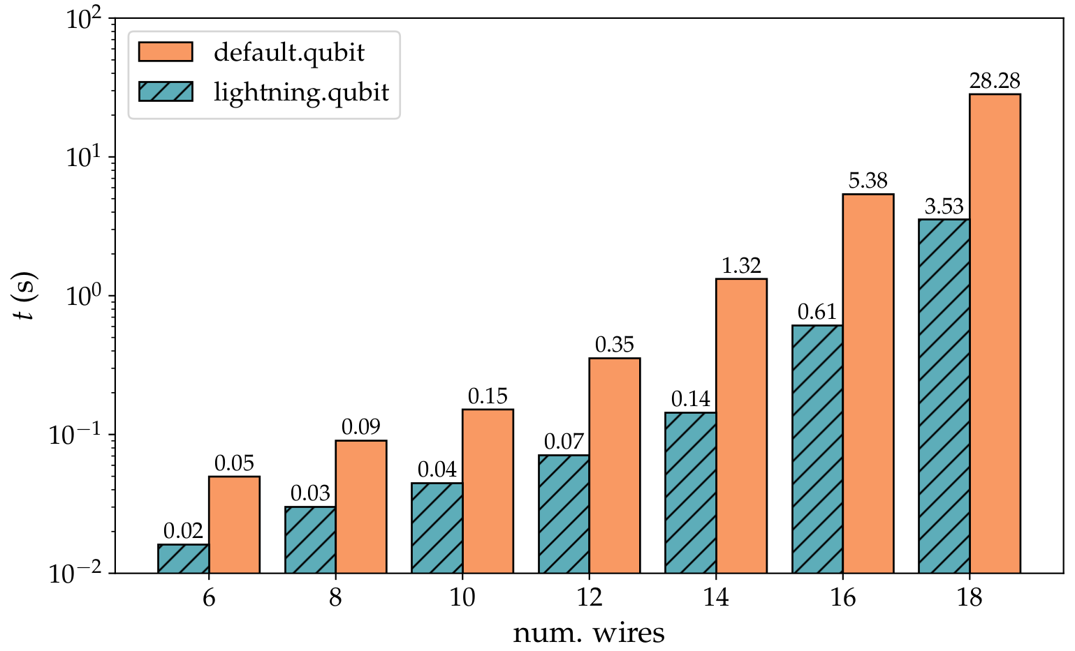
Support for native backpropagation using PyTorch
The built-in PennyLane simulator
default.qubitnow supports backpropogation with PyTorch. (#1360) (#1598)As a result,
default.qubitcan now use end-to-end classical backpropagation as a means to compute gradients. End-to-end backpropagation can be faster than the parameter-shift rule for computing quantum gradients when the number of parameters to be optimized is large. This is now the default differentiation method when usingdefault.qubitwith PyTorch.Using this method, the created QNode is a ‘white-box’ that is tightly integrated with your PyTorch computation, including TorchScript and GPU support.
x = torch.tensor(0.43316321, dtype=torch.float64, requires_grad=True) y = torch.tensor(0.2162158, dtype=torch.float64, requires_grad=True) z = torch.tensor(0.75110998, dtype=torch.float64, requires_grad=True) p = torch.tensor([x, y, z], requires_grad=True) dev = qml.device("default.qubit", wires=1) @qml.qnode(dev, interface="torch", diff_method="backprop") def circuit(x): qml.Rot(x[0], x[1], x[2], wires=0) return qml.expval(qml.PauliZ(0)) res = circuit(p) res.backward()
>>> res = circuit(p) >>> res.backward() >>> print(p.grad) tensor([-9.1798e-17, -2.1454e-01, -1.0511e-16], dtype=torch.float64)
Improved quantum optimization methods
The
RotosolveOptimizernow can tackle general parametrized circuits, and is no longer restricted to single-qubit Pauli rotations. (#1489)This includes:
layers of gates controlled by the same parameter,
controlled variants of parametrized gates, and
Hamiltonian time evolution.
Note that the eigenvalue spectrum of the gate generator needs to be known to use
RotosolveOptimizerfor a general gate, and it is required to produce equidistant frequencies. For details see Vidal and Theis, 2018 and Wierichs, Izaac, Wang, Lin 2021.Consider a circuit with a mixture of Pauli rotation gates, controlled Pauli rotations, and single-parameter layers of Pauli rotations:
dev = qml.device('default.qubit', wires=3, shots=None) @qml.qnode(dev) def cost_function(rot_param, layer_par, crot_param): for i, par in enumerate(rot_param): qml.RX(par, wires=i) for w in dev.wires: qml.RX(layer_par, wires=w) for i, par in enumerate(crot_param): qml.CRY(par, wires=[i, (i+1) % 3]) return qml.expval(qml.PauliZ(0) @ qml.PauliZ(1) @ qml.PauliZ(2))
This cost function has one frequency for each of the first
RXrotation angles, three frequencies for the layer ofRXgates that depend onlayer_par, and two frequencies for each of theCRYgate parameters. Rotosolve can then be used to minimize thecost_function:# Initial parameters init_param = [ np.array([0.3, 0.2, 0.67], requires_grad=True), np.array(1.1, requires_grad=True), np.array([-0.2, 0.1, -2.5], requires_grad=True), ] # Numbers of frequencies per parameter num_freqs = [[1, 1, 1], 3, [2, 2, 2]] opt = qml.RotosolveOptimizer() param = init_param.copy()
In addition, the optimization technique for the Rotosolve substeps can be chosen via the
optimizerandoptimizer_kwargskeyword arguments and the minimized cost of the intermediate univariate reconstructions can be read out viafull_output, including the cost after the full Rotosolve step:for step in range(3): param, cost, sub_cost = opt.step_and_cost( cost_function, *param, num_freqs=num_freqs, full_output=True, optimizer="brute", ) print(f"Cost before step: {cost}") print(f"Minimization substeps: {np.round(sub_cost, 6)}")
Cost before step: 0.042008210392535605 Minimization substeps: [-0.230905 -0.863336 -0.980072 -0.980072 -1. -1. -1. ] Cost before step: -0.999999999068121 Minimization substeps: [-1. -1. -1. -1. -1. -1. -1.] Cost before step: -1.0 Minimization substeps: [-1. -1. -1. -1. -1. -1. -1.]
For usage details please consider the docstring of the optimizer.
Faster, trainable, Hamiltonian simulations
Hamiltonians are now trainable with respect to their coefficients. (#1483)
from pennylane import numpy as np dev = qml.device("default.qubit", wires=2) @qml.qnode(dev) def circuit(coeffs, param): qml.RX(param, wires=0) qml.RY(param, wires=0) return qml.expval( qml.Hamiltonian(coeffs, [qml.PauliX(0), qml.PauliZ(0)], simplify=True) ) coeffs = np.array([-0.05, 0.17]) param = np.array(1.7) grad_fn = qml.grad(circuit)
>>> grad_fn(coeffs, param) (array([-0.12777055, 0.0166009 ]), array(0.0917819))
Furthermore, a gradient recipe for Hamiltonian coefficients has been added. This makes it possible to compute parameter-shift gradients of these coefficients on devices that natively support Hamiltonians. (#1551)
Hamiltonians are now natively supported on the
default.qubitdevice ifshots=None. This makes VQE workflows a lot faster in some cases. (#1551) (#1596)
The Hamiltonian can now store grouping information, which can be accessed by a device to speed up computations of the expectation value of a Hamiltonian. (#1515)
obs = [qml.PauliX(0), qml.PauliX(1), qml.PauliZ(0)] coeffs = np.array([1., 2., 3.]) H = qml.Hamiltonian(coeffs, obs, grouping_type='qwc')
Initialization with a
grouping_typeother thanNonestores the indices required to make groups of commuting observables and their coefficients.>>> H.grouping_indices [[0, 1], [2]]
Create multi-circuit quantum transforms and custom gradient rules
Custom gradient transforms can now be created using the new
@qml.gradients.gradient_transformdecorator on a batch-tape transform. (#1589)Quantum gradient transforms are a specific case of
qml.batch_transform.Supported gradient transforms must be of the following form:
@qml.gradients.gradient_transform def my_custom_gradient(tape, argnum=None, **kwargs): ... return gradient_tapes, processing_fn
Various built-in quantum gradient transforms are provided within the
qml.gradientsmodule, includingqml.gradients.param_shift. Once defined, quantum gradient transforms can be applied directly to QNodes:>>> @qml.qnode(dev) ... def circuit(x): ... qml.RX(x, wires=0) ... qml.CNOT(wires=[0, 1]) ... return qml.expval(qml.PauliZ(0)) >>> circuit(0.3) tensor(0.95533649, requires_grad=True) >>> qml.gradients.param_shift(circuit)(0.5) array([[-0.47942554]])
Quantum gradient transforms are fully differentiable, allowing higher order derivatives to be accessed:
>>> qml.grad(qml.gradients.param_shift(circuit))(0.5) tensor(-0.87758256, requires_grad=True)
Refer to the page of quantum gradient transforms for more details.
The ability to define batch transforms has been added via the new
@qml.batch_transformdecorator. (#1493)A batch transform is a transform that takes a single tape or QNode as input, and executes multiple tapes or QNodes independently. The results may then be post-processed before being returned.
For example, consider the following batch transform:
@qml.batch_transform def my_transform(tape, a, b): """Generates two tapes, one with all RX replaced with RY, and the other with all RX replaced with RZ.""" tape1 = qml.tape.JacobianTape() tape2 = qml.tape.JacobianTape() # loop through all operations on the input tape for op in tape.operations + tape.measurements: if op.name == "RX": with tape1: qml.RY(a * qml.math.abs(op.parameters[0]), wires=op.wires) with tape2: qml.RZ(b * qml.math.abs(op.parameters[0]), wires=op.wires) else: for t in [tape1, tape2]: with t: qml.apply(op) def processing_fn(results): return qml.math.sum(qml.math.stack(results)) return [tape1, tape2], processing_fn
We can transform a QNode directly using decorator syntax:
>>> @my_transform(0.65, 2.5) ... @qml.qnode(dev) ... def circuit(x): ... qml.Hadamard(wires=0) ... qml.RX(x, wires=0) ... return qml.expval(qml.PauliX(0)) >>> print(circuit(-0.5)) 1.2629730888100839
Batch tape transforms are fully differentiable:
>>> gradient = qml.grad(circuit)(-0.5) >>> print(gradient) 2.5800122591960153
Batch transforms can also be applied to existing QNodes,
>>> new_qnode = my_transform(existing_qnode, *transform_weights) >>> new_qnode(weights)
or to tapes (in which case, the processed tapes and classical post-processing functions are returned):
>>> tapes, fn = my_transform(tape, 0.65, 2.5) >>> from pennylane.interfaces.batch import execute >>> dev = qml.device("default.qubit", wires=1) >>> res = execute(tapes, dev, interface="autograd", gradient_fn=qml.gradients.param_shift) 1.2629730888100839
Vector-Jacobian product transforms have been added to the
qml.gradientspackage. (#1494)The new transforms include:
qml.gradients.vjpqml.gradients.batch_vjp
Support for differentiable execution of batches of circuits has been added, via the beta
pennylane.interfaces.batchmodule. (#1501) (#1508) (#1542) (#1549) (#1608) (#1618) (#1637)For now, this is a low-level feature, and will be integrated into the QNode in a future release. For example:
from pennylane.interfaces.batch import execute def cost_fn(x): with qml.tape.JacobianTape() as tape1: qml.RX(x[0], wires=[0]) qml.RY(x[1], wires=[1]) qml.CNOT(wires=[0, 1]) qml.var(qml.PauliZ(0) @ qml.PauliX(1)) with qml.tape.JacobianTape() as tape2: qml.RX(x[0], wires=0) qml.RY(x[0], wires=1) qml.CNOT(wires=[0, 1]) qml.probs(wires=1) result = execute( [tape1, tape2], dev, gradient_fn=qml.gradients.param_shift, interface="autograd" ) return result[0] + result[1][0, 0] res = qml.grad(cost_fn)(params)
Improvements
A new operation
qml.SISWAPhas been added, the square-root of theqml.ISWAPoperation. (#1563)The
frobenius_inner_productfunction has been moved to theqml.mathmodule, and is now differentiable using all autodiff frameworks. (#1388)A warning is raised to inform the user that specifying a list of shots is only supported for
QubitDevicebased devices. (#1659)The
qml.circuit_drawer.MPLDrawerclass provides manual circuit drawing functionality using Matplotlib. While not yet integrated with automatic circuit drawing, this class provides customization and control. (#1484)from pennylane.circuit_drawer import MPLDrawer drawer = MPLDrawer(n_wires=3, n_layers=3) drawer.label([r"$|\Psi\rangle$", r"$|\theta\rangle$", "aux"]) drawer.box_gate(layer=0, wires=[0, 1, 2], text="Entangling Layers", text_options={'rotation': 'vertical'}) drawer.box_gate(layer=1, wires=[0, 1], text="U(θ)") drawer.CNOT(layer=2, wires=[1, 2]) drawer.measure(layer=3, wires=2) drawer.fig.suptitle('My Circuit', fontsize='xx-large')

The slowest tests, more than 1.5 seconds, now have the pytest mark
slow, and can be selected or deselected during local execution of tests. (#1633)The device test suite has been expanded to cover more qubit operations and observables. (#1510)
The
MultiControlledXclass now inherits fromOperationinstead ofControlledQubitUnitarywhich makes theMultiControlledXgate a non-parameterized gate. (#1557)The
utils.sparse_hamiltonianfunction can now deal with non-integer wire labels, and it throws an error for the edge case of observables that are created from multi-qubit operations. (#1550)Added the matrix attribute to
qml.templates.subroutines.GroverOperator(#1553)The
tape.to_openqasm()method now has ameasure_allargument that specifies whether the serialized OpenQASM script includes computational basis measurements on all of the qubits or just those specified by the tape. (#1559)An error is now raised when no arguments are passed to an observable, to inform that wires have not been supplied. (#1547)
The
group_observablestransform is now differentiable. (#1483)For example:
import jax from jax import numpy as jnp coeffs = jnp.array([1., 2., 3.]) obs = [PauliX(wires=0), PauliX(wires=1), PauliZ(wires=1)] def group(coeffs, select=None): _, grouped_coeffs = qml.grouping.group_observables(obs, coeffs) # in this example, grouped_coeffs is a list of two jax tensors # [Array([1., 2.], dtype=float32), Array([3.], dtype=float32)] return grouped_coeffs[select] jac_fn = jax.jacobian(group)
>>> jac_fn(coeffs, select=0) [[1. 0. 0.] [0. 1. 0.]] >>> jac_fn(coeffs, select=1) [[0., 0., 1.]]
The tape does not verify any more that all Observables have owners in the annotated queue. (#1505)
This allows manipulation of Observables inside a tape context. An example is
expval(Tensor(qml.PauliX(0), qml.Identity(1)).prune())which makes the expval an owner of the pruned tensor and its constituent observables, but leaves the original tensor in the queue without an owner.The
qml.ResetErroris now supported fordefault.mixeddevice. (#1541)QNode.diff_methodwill now reflect which method was selected fromdiff_method="best". (#1568)QNodes now support
diff_method=None. This works the same asinterface=None. Such QNodes accept floats, ints, lists and NumPy arrays and return NumPy output but can not be differentiated. (#1585)QNodes now include validation to warn users if a supplied keyword argument is not one of the recognized arguments. (#1591)
Breaking changes
The
QFToperation has been moved, and is now accessible viapennylane.templates.QFT. (#1548)Specifying
shots=Nonewithqml.samplewas previously deprecated. From this release onwards, settingshots=Nonewhen sampling will raise an error also fordefault.qubit.jax. (#1629)An error is raised during QNode creation when a user requests backpropagation on a device with finite-shots. (#1588)
The class
qml.Interferometeris deprecated and will be renamedqml.InterferometerUnitaryafter one release cycle. (#1546)All optimizers except for Rotosolve and Rotoselect now have a public attribute
stepsize. Temporary backward compatibility has been added to support the use of_stepsizefor one release cycle.update_stepsizemethod is deprecated. (#1625)
Bug fixes
Fixed a bug with shot vectors and
Devicebase class. (#1666)Fixed a bug where
@jax.jitwould fail on a QNode that usedqml.QubitStateVector. (#1649)Fixed a bug related to an edge case of single-qubit
zyz_decompositionwhen only off-diagonal elements are present. (#1643)MottonenStatepreparationcan now be run with a single wire label not in a list. (#1620)Fixed the circuit representation of CY gates to align with CNOT and CZ gates when calling the circuit drawer. (#1504)
Dask and CVXPY dependent tests are skipped if those packages are not installed. (#1617)
The
qml.layertemplate now works with tensorflow variables. (#1615)Remove
QFTfrom possible operations indefault.qubitanddefault.mixed. (#1600)Fixed a bug when computing expectations of Hamiltonians using TensorFlow. (#1586)
Fixed a bug when computing the specs of a circuit with a Hamiltonian observable. (#1533)
Documentation
The
qml.Identityoperation is placed under the sections Qubit observables and CV observables. (#1576)Updated the documentation of
qml.grouping,qml.kernelsandqml.qaoamodules to present the list of functions first followed by the technical details of the module. (#1581)Recategorized Qubit operations into new and existing categories so that code for each operation is easier to locate. (#1566)
Contributors
This release contains contributions from (in alphabetical order):
Vishnu Ajith, Akash Narayanan B, Thomas Bromley, Olivia Di Matteo, Sahaj Dhamija, Tanya Garg, Anthony Hayes, Theodor Isacsson, Josh Izaac, Prateek Jain, Ankit Khandelwal, Nathan Killoran, Christina Lee, Ian McLean, Johannes Jakob Meyer, Romain Moyard, Lee James O’Riordan, Esteban Payares, Pratul Saini, Maria Schuld, Arshpreet Singh, Jay Soni, Ingrid Strandberg, Antal Száva, Slimane Thabet, David Wierichs, Vincent Wong.
- orphan
Release 0.17.0¶
New features since the last release
Circuit optimization
PennyLane can now perform quantum circuit optimization using the top-level transform
qml.compile. Thecompiletransform allows you to chain together sequences of tape and quantum function transforms into custom circuit optimization pipelines. (#1475)For example, take the following decorated quantum function:
dev = qml.device('default.qubit', wires=[0, 1, 2]) @qml.qnode(dev) @qml.compile() def qfunc(x, y, z): qml.Hadamard(wires=0) qml.Hadamard(wires=1) qml.Hadamard(wires=2) qml.RZ(z, wires=2) qml.CNOT(wires=[2, 1]) qml.RX(z, wires=0) qml.CNOT(wires=[1, 0]) qml.RX(x, wires=0) qml.CNOT(wires=[1, 0]) qml.RZ(-z, wires=2) qml.RX(y, wires=2) qml.PauliY(wires=2) qml.CZ(wires=[1, 2]) return qml.expval(qml.PauliZ(wires=0))
The default behaviour of
qml.compileis to apply a sequence of three transforms:commute_controlled,cancel_inverses, and thenmerge_rotations.>>> print(qml.draw(qfunc)(0.2, 0.3, 0.4)) 0: ──H───RX(0.6)──────────────────┤ ⟨Z⟩ 1: ──H──╭X────────────────────╭C──┤ 2: ──H──╰C────────RX(0.3)──Y──╰Z──┤
The
qml.compiletransform is flexible and accepts a custom pipeline of tape and quantum function transforms (you can even write your own!). For example, if we wanted to only push single-qubit gates through controlled gates and cancel adjacent inverses, we could do:from pennylane.transforms import commute_controlled, cancel_inverses pipeline = [commute_controlled, cancel_inverses] @qml.qnode(dev) @qml.compile(pipeline=pipeline) def qfunc(x, y, z): qml.Hadamard(wires=0) qml.Hadamard(wires=1) qml.Hadamard(wires=2) qml.RZ(z, wires=2) qml.CNOT(wires=[2, 1]) qml.RX(z, wires=0) qml.CNOT(wires=[1, 0]) qml.RX(x, wires=0) qml.CNOT(wires=[1, 0]) qml.RZ(-z, wires=2) qml.RX(y, wires=2) qml.PauliY(wires=2) qml.CZ(wires=[1, 2]) return qml.expval(qml.PauliZ(wires=0))
>>> print(qml.draw(qfunc)(0.2, 0.3, 0.4)) 0: ──H───RX(0.4)──RX(0.2)────────────────────────────┤ ⟨Z⟩ 1: ──H──╭X───────────────────────────────────────╭C──┤ 2: ──H──╰C────────RZ(0.4)──RZ(-0.4)──RX(0.3)──Y──╰Z──┤
The following compilation transforms have been added and are also available to use, either independently, or within a
qml.compilepipeline:commute_controlled: push commuting single-qubit gates through controlled operations. (#1464)cancel_inverses: removes adjacent pairs of operations that cancel out. (#1455)merge_rotations: combines adjacent rotation gates of the same type into a single gate, including controlled rotations. (#1455)single_qubit_fusion: acts on all sequences of single-qubit operations in a quantum function, and converts each sequence to a singleRotgate. (#1458)
For more details on
qml.compileand the available compilation transforms, see the compilation documentation.
QNodes are even more powerful
Computational basis samples directly from the underlying device can now be returned directly from QNodes via
qml.sample(). (#1441)dev = qml.device("default.qubit", wires=3, shots=5) @qml.qnode(dev) def circuit_1(): qml.Hadamard(wires=0) qml.Hadamard(wires=1) return qml.sample() @qml.qnode(dev) def circuit_2(): qml.Hadamard(wires=0) qml.Hadamard(wires=1) return qml.sample(wires=[0,2]) # no observable provided and wires specified
>>> print(circuit_1()) [[1, 0, 0], [1, 1, 0], [1, 0, 0], [0, 0, 0], [0, 1, 0]] >>> print(circuit_2()) [[1, 0], [1, 0], [1, 0], [0, 0], [0, 0]] >>> print(qml.draw(circuit_2)()) 0: ──H──╭┤ Sample[basis] 1: ──H──│┤ 2: ─────╰┤ Sample[basis]
The new
qml.applyfunction can be used to add operations that might have already been instantiated elsewhere to the QNode and other queuing contexts: (#1433)op = qml.RX(0.4, wires=0) dev = qml.device("default.qubit", wires=2) @qml.qnode(dev) def circuit(x): qml.RY(x, wires=0) qml.apply(op) return qml.expval(qml.PauliZ(0))
>>> print(qml.draw(circuit)(0.6)) 0: ──RY(0.6)──RX(0.4)──┤ ⟨Z⟩
Previously instantiated measurements can also be applied to QNodes.
Device Resource Tracker
The new Device Tracker capabilities allows for flexible and versatile tracking of executions, even inside parameter-shift gradients. This functionality will improve the ease of monitoring large batches and remote jobs. (#1355)
dev = qml.device('default.qubit', wires=1, shots=100) @qml.qnode(dev, diff_method="parameter-shift") def circuit(x): qml.RX(x, wires=0) return qml.expval(qml.PauliZ(0)) x = np.array(0.1) with qml.Tracker(circuit.device) as tracker: qml.grad(circuit)(x)
>>> tracker.totals {'executions': 3, 'shots': 300, 'batches': 1, 'batch_len': 2} >>> tracker.history {'executions': [1, 1, 1], 'shots': [100, 100, 100], 'batches': [1], 'batch_len': [2]} >>> tracker.latest {'batches': 1, 'batch_len': 2}
Users can also provide a custom function to the
callbackkeyword that gets called each time the information is updated. This functionality allows users to monitor remote jobs or large parameter-shift batches.>>> def shots_info(totals, history, latest): ... print("Total shots: ", totals['shots']) >>> with qml.Tracker(circuit.device, callback=shots_info) as tracker: ... qml.grad(circuit)(0.1) Total shots: 100 Total shots: 200 Total shots: 300 Total shots: 300
Containerization support
Docker support for building PennyLane with support for all interfaces (TensorFlow, Torch, and Jax), as well as device plugins and QChem, for GPUs and CPUs, has been added. (#1391)
The build process using Docker and
makerequires that the repository source code is cloned or downloaded from GitHub. Visit the the detailed description for an extended list of options.
Improved Hamiltonian simulations
Added a sparse Hamiltonian observable and the functionality to support computing its expectation value with
default.qubit. (#1398)For example, the following QNode returns the expectation value of a sparse Hamiltonian:
dev = qml.device("default.qubit", wires=2) @qml.qnode(dev, diff_method="parameter-shift") def circuit(param, H): qml.PauliX(0) qml.SingleExcitation(param, wires=[0, 1]) return qml.expval(qml.SparseHamiltonian(H, [0, 1]))
We can execute this QNode, passing in a sparse identity matrix:
>>> print(circuit([0.5], scipy.sparse.eye(4).tocoo())) 0.9999999999999999
The expectation value of the sparse Hamiltonian is computed directly, which leads to executions that are faster by orders of magnitude. Note that “parameter-shift” is the only differentiation method that is currently supported when the observable is a sparse Hamiltonian.
VQE problems can now be intuitively set up by passing the Hamiltonian as an observable. (#1474)
dev = qml.device("default.qubit", wires=2) H = qml.Hamiltonian([1., 2., 3.], [qml.PauliZ(0), qml.PauliY(0), qml.PauliZ(1)]) w = qml.init.strong_ent_layers_uniform(1, 2, seed=1967) @qml.qnode(dev) def circuit(w): qml.templates.StronglyEntanglingLayers(w, wires=range(2)) return qml.expval(H)
>>> print(circuit(w)) -1.5133943637878295 >>> print(qml.grad(circuit)(w)) [[[-8.32667268e-17 1.39122955e+00 -9.12462052e-02] [ 1.02348685e-16 -7.77143238e-01 -1.74708049e-01]]]
Note that other measurement types like
var(H)orsample(H), as well as multiple expectations likeexpval(H1), expval(H2)are not supported.Added functionality to compute the sparse matrix representation of a
qml.Hamiltonianobject. (#1394)
New gradients module
A new gradients module
qml.gradientshas been added, which provides differentiable quantum gradient transforms. (#1476) (#1479) (#1486)Available quantum gradient transforms include:
qml.gradients.finite_diffqml.gradients.param_shiftqml.gradients.param_shift_cv
For example,
>>> params = np.array([0.3,0.4,0.5], requires_grad=True) >>> with qml.tape.JacobianTape() as tape: ... qml.RX(params[0], wires=0) ... qml.RY(params[1], wires=0) ... qml.RX(params[2], wires=0) ... qml.expval(qml.PauliZ(0)) ... qml.var(qml.PauliZ(0)) >>> tape.trainable_params = {0, 1, 2} >>> gradient_tapes, fn = qml.gradients.finite_diff(tape) >>> res = dev.batch_execute(gradient_tapes) >>> fn(res) array([[-0.69688381, -0.32648317, -0.68120105], [ 0.8788057 , 0.41171179, 0.85902895]])
Even more new operations and templates
Grover Diffusion Operator template added. (#1442)
For example, if we have an oracle that marks the “all ones” state with a negative sign:
n_wires = 3 wires = list(range(n_wires)) def oracle(): qml.Hadamard(wires[-1]) qml.Toffoli(wires=wires) qml.Hadamard(wires[-1])
We can perform Grover’s Search Algorithm:
dev = qml.device('default.qubit', wires=wires) @qml.qnode(dev) def GroverSearch(num_iterations=1): for wire in wires: qml.Hadamard(wire) for _ in range(num_iterations): oracle() qml.templates.GroverOperator(wires=wires) return qml.probs(wires)
We can see this circuit yields the marked state with high probability:
>>> GroverSearch(num_iterations=1) tensor([0.03125, 0.03125, 0.03125, 0.03125, 0.03125, 0.03125, 0.03125, 0.78125], requires_grad=True) >>> GroverSearch(num_iterations=2) tensor([0.0078125, 0.0078125, 0.0078125, 0.0078125, 0.0078125, 0.0078125, 0.0078125, 0.9453125], requires_grad=True)
A decomposition has been added to
QubitUnitarythat makes the single-qubit case fully differentiable in all interfaces. Furthermore, a quantum function transform,unitary_to_rot(), has been added to decompose all single-qubit instances ofQubitUnitaryin a quantum circuit. (#1427)Instances of
QubitUnitarymay now be decomposed directly toRotoperations, orRZoperations if the input matrix is diagonal. For example, let>>> U = np.array([ [-0.28829348-0.78829734j, 0.30364367+0.45085995j], [ 0.53396245-0.10177564j, 0.76279558-0.35024096j] ])
Then, we can compute the decomposition as:
>>> qml.QubitUnitary.decomposition(U, wires=0) [Rot(-0.24209530281458358, 1.1493817777199102, 1.733058145303424, wires=[0])]
We can also apply the transform directly to a quantum function, and compute the gradients of parameters used to construct the unitary matrices.
def qfunc_with_qubit_unitary(angles): z, x = angles[0], angles[1] Z_mat = np.array([[np.exp(-1j * z / 2), 0.0], [0.0, np.exp(1j * z / 2)]]) c = np.cos(x / 2) s = np.sin(x / 2) * 1j X_mat = np.array([[c, -s], [-s, c]]) qml.Hadamard(wires="a") qml.QubitUnitary(Z_mat, wires="a") qml.QubitUnitary(X_mat, wires="b") qml.CNOT(wires=["b", "a"]) return qml.expval(qml.PauliX(wires="a"))
>>> dev = qml.device("default.qubit", wires=["a", "b"]) >>> transformed_qfunc = qml.transforms.unitary_to_rot(qfunc_with_qubit_unitary) >>> transformed_qnode = qml.QNode(transformed_qfunc, dev) >>> input = np.array([0.3, 0.4], requires_grad=True) >>> transformed_qnode(input) tensor(0.95533649, requires_grad=True) >>> qml.grad(transformed_qnode)(input) array([-0.29552021, 0. ])
Ising YY gate functionality added. (#1358)
Improvements
The tape does not verify any more that all Observables have owners in the annotated queue. (#1505)
This allows manipulation of Observables inside a tape context. An example is
expval(Tensor(qml.PauliX(0), qml.Identity(1)).prune())which makes the expval an owner of the pruned tensor and its constituent observables, but leaves the original tensor in the queue without an owner.The
stepandstep_and_costmethods ofQNGOptimizernow accept a customgrad_fnkeyword argument to use for gradient computations. (#1487)The precision used by
default.qubit.jaxnow matches the float precision indicated byfrom jax.config import config config.read('jax_enable_x64')
where
Truemeansfloat64/complex128andFalsemeansfloat32/complex64. (#1485)The
./pennylane/ops/qubit.pyfile is broken up into a folder of six separate files. (#1467)Changed to using commas as the separator of wires in the string representation of
qml.Hamiltonianobjects for multi-qubit terms. (#1465)Changed to using
np.object_instead ofnp.objectas per the NumPy deprecations starting version 1.20. (#1466)Change the order of the covariance matrix and the vector of means internally in
default.gaussian. (#1331)Added the
idattribute to templates. (#1438)The
qml.mathmodule, for framework-agnostic tensor manipulation, has two new functions available: (#1490)qml.math.get_trainable_indices(sequence_of_tensors): returns the indices corresponding to trainable tensors in the input sequence.qml.math.unwrap(sequence_of_tensors): unwraps a sequence of tensor-like objects to NumPy arrays.
In addition, the behaviour of
qml.math.requires_gradhas been improved in order to correctly determine trainability during Autograd and JAX backwards passes.A new tape method,
tape.unwrap()is added. This method is a context manager; inside the context, the tape’s parameters are unwrapped to NumPy arrays and floats, and the trainable parameter indices are set. (#1491)These changes are temporary, and reverted on exiting the context.
>>> with tf.GradientTape(): ... with qml.tape.QuantumTape() as tape: ... qml.RX(tf.Variable(0.1), wires=0) ... qml.RY(tf.constant(0.2), wires=0) ... qml.RZ(tf.Variable(0.3), wires=0) ... with tape.unwrap(): ... print("Trainable params:", tape.trainable_params) ... print("Unwrapped params:", tape.get_parameters()) Trainable params: {0, 2} Unwrapped params: [0.1, 0.3] >>> print("Original parameters:", tape.get_parameters()) Original parameters: [<tf.Variable 'Variable:0' shape=() dtype=float32, numpy=0.1>, <tf.Variable 'Variable:0' shape=() dtype=float32, numpy=0.3>]
In addition,
qml.tape.Unwrapis a context manager that unwraps multiple tapes:>>> with qml.tape.Unwrap(tape1, tape2):
Breaking changes
Removed the deprecated tape methods
get_resourcesandget_depthas they are superseded by thespecstape attribute. (#1522)Specifying
shots=Nonewithqml.samplewas previously deprecated. From this release onwards, settingshots=Nonewhen sampling will raise an error. (#1522)The existing
pennylane.collections.applyfunction is no longer accessible viaqml.apply, and needs to be imported directly from thecollectionspackage. (#1358)
Bug fixes
Fixes a bug in
qml.adjointandqml.ctrlwhere the adjoint of operations outside of aQNodeor aQuantumTapecould not be obtained. (#1532)Fixes a bug in
GradientDescentOptimizerandNesterovMomentumOptimizerwhere a cost function with one trainable parameter and non-trainable parameters raised an error. (#1495)Fixed an example in the documentation’s introduction to numpy gradients, where the wires were a non-differentiable argument to the QNode. (#1499)
Fixed a bug where the adjoint of
qml.QFTwhen using theqml.adjointfunction was not correctly computed. (#1451)Fixed the differentiability of the operation
IsingYYfor Autograd, Jax and Tensorflow. (#1425)Fixed a bug in the
torchinterface that prevented gradients from being computed on a GPU. (#1426)Quantum function transforms now preserve the format of the measurement results, so that a single measurement returns a single value rather than an array with a single element. (#1434)
Fixed a bug in the parameter-shift Hessian implementation, which resulted in the incorrect Hessian being returned for a cost function that performed post-processing on a vector-valued QNode. (#1436)
Fixed a bug in the initialization of
QubitUnitarywhere the size of the matrix was not checked against the number of wires. (#1439)
Documentation
Improved Contribution Guide and Pull Requests Guide. (#1461)
Examples have been added to clarify use of the continuous-variable
FockStateVectoroperation in the multi-mode case. (#1472)
Contributors
This release contains contributions from (in alphabetical order):
Juan Miguel Arrazola, Olivia Di Matteo, Anthony Hayes, Theodor Isacsson, Josh Izaac, Soran Jahangiri, Nathan Killoran, Arshpreet Singh Khangura, Leonhard Kunczik, Christina Lee, Romain Moyard, Lee James O’Riordan, Ashish Panigrahi, Nahum Sá, Maria Schuld, Jay Soni, Antal Száva, David Wierichs.
- orphan
Release 0.16.0¶
First class support for quantum kernels
The new
qml.kernelsmodule provides basic functionalities for working with quantum kernels as well as post-processing methods to mitigate sampling errors and device noise: (#1102)num_wires = 6 wires = range(num_wires) dev = qml.device('default.qubit', wires=wires) @qml.qnode(dev) def kernel_circuit(x1, x2): qml.templates.AngleEmbedding(x1, wires=wires) qml.adjoint(qml.templates.AngleEmbedding)(x2, wires=wires) return qml.probs(wires) kernel = lambda x1, x2: kernel_circuit(x1, x2)[0] X_train = np.random.random((10, 6)) X_test = np.random.random((5, 6)) # Create symmetric square kernel matrix (for training) K = qml.kernels.square_kernel_matrix(X_train, kernel) # Compute kernel between test and training data. K_test = qml.kernels.kernel_matrix(X_train, X_test, kernel) K1 = qml.kernels.mitigate_depolarizing_noise(K, num_wires, method='single')
Extract the fourier representation of quantum circuits
PennyLane now has a
fouriermodule, which hosts a growing library of methods that help with investigating the Fourier representation of functions implemented by quantum circuits. The Fourier representation can be used to examine and characterize the expressivity of the quantum circuit. (#1160) (#1378)For example, one can plot distributions over Fourier series coefficients like this one:

Seamless support for working with the Pauli group
Added functionality for constructing and manipulating the Pauli group (#1181).
The function
qml.grouping.pauli_groupprovides a generator to easily loop over the group, or construct and store it in its entirety. For example, we can construct the single-qubit Pauli group like so:>>> from pennylane.grouping import pauli_group >>> pauli_group_1_qubit = list(pauli_group(1)) >>> pauli_group_1_qubit [Identity(wires=[0]), PauliZ(wires=[0]), PauliX(wires=[0]), PauliY(wires=[0])]
We can multiply together its members at the level of Pauli words using the
pauli_multandpauli_multi_with_phasefunctions. This can be done on arbitrarily-labeled wires as well, by defining a wire map.>>> from pennylane.grouping import pauli_group, pauli_mult >>> wire_map = {'a' : 0, 'b' : 1, 'c' : 2} >>> pg = list(pauli_group(3, wire_map=wire_map)) >>> pg[3] PauliZ(wires=['b']) @ PauliZ(wires=['c']) >>> pg[55] PauliY(wires=['a']) @ PauliY(wires=['b']) @ PauliZ(wires=['c']) >>> pauli_mult(pg[3], pg[55], wire_map=wire_map) PauliY(wires=['a']) @ PauliX(wires=['b'])
Functions for conversion of Pauli observables to strings (and back), are included.
>>> from pennylane.grouping import pauli_word_to_string, string_to_pauli_word >>> pauli_word_to_string(pg[55], wire_map=wire_map) 'YYZ' >>> string_to_pauli_word('ZXY', wire_map=wire_map) PauliZ(wires=['a']) @ PauliX(wires=['b']) @ PauliY(wires=['c'])
Calculation of the matrix representation for arbitrary Paulis and wire maps is now also supported.
>>> from pennylane.grouping import pauli_word_to_matrix >>> wire_map = {'a' : 0, 'b' : 1} >>> pauli_word = qml.PauliZ('b') # corresponds to Pauli 'IZ' >>> pauli_word_to_matrix(pauli_word, wire_map=wire_map) array([[ 1., 0., 0., 0.], [ 0., -1., 0., -0.], [ 0., 0., 1., 0.], [ 0., -0., 0., -1.]])
New transforms
The
qml.specsQNode transform creates a function that returns specifications or details about the QNode, including depth, number of gates, and number of gradient executions required. (#1245)For example:
dev = qml.device('default.qubit', wires=4) @qml.qnode(dev, diff_method='parameter-shift') def circuit(x, y): qml.RX(x[0], wires=0) qml.Toffoli(wires=(0, 1, 2)) qml.CRY(x[1], wires=(0, 1)) qml.Rot(x[2], x[3], y, wires=0) return qml.expval(qml.PauliZ(0)), qml.expval(qml.PauliX(1))
We can now use the
qml.specstransform to generate a function that returns details and resource information:>>> x = np.array([0.05, 0.1, 0.2, 0.3], requires_grad=True) >>> y = np.array(0.4, requires_grad=False) >>> specs_func = qml.specs(circuit) >>> specs_func(x, y) {'gate_sizes': defaultdict(int, {1: 2, 3: 1, 2: 1}), 'gate_types': defaultdict(int, {'RX': 1, 'Toffoli': 1, 'CRY': 1, 'Rot': 1}), 'num_operations': 4, 'num_observables': 2, 'num_diagonalizing_gates': 1, 'num_used_wires': 3, 'depth': 4, 'num_trainable_params': 4, 'num_parameter_shift_executions': 11, 'num_device_wires': 4, 'device_name': 'default.qubit', 'diff_method': 'parameter-shift'}
The tape methods
get_resourcesandget_depthare superseded byspecsand will be deprecated after one release cycle.Adds a decorator
@qml.qfunc_transformto easily create a transformation that modifies the behaviour of a quantum function. (#1315)For example, consider the following transform, which scales the parameter of all
RXgates by \(x \rightarrow \sin(a) \sqrt{x}\), and the parameters of allRYgates by \(y \rightarrow \cos(a * b) y\):@qml.qfunc_transform def my_transform(tape, a, b): for op in tape.operations + tape.measurements: if op.name == "RX": x = op.parameters[0] qml.RX(qml.math.sin(a) * qml.math.sqrt(x), wires=op.wires) elif op.name == "RY": y = op.parameters[0] qml.RX(qml.math.cos(a * b) * y, wires=op.wires) else: op.queue()
We can now apply this transform to any quantum function:
dev = qml.device("default.qubit", wires=2) def ansatz(x): qml.Hadamard(wires=0) qml.RX(x[0], wires=0) qml.RY(x[1], wires=1) qml.CNOT(wires=[0, 1]) @qml.qnode(dev) def circuit(params, transform_weights): qml.RX(0.1, wires=0) # apply the transform to the ansatz my_transform(*transform_weights)(ansatz)(params) return qml.expval(qml.PauliZ(1))
We can print this QNode to show that the qfunc transform is taking place:
>>> x = np.array([0.5, 0.3], requires_grad=True) >>> transform_weights = np.array([0.1, 0.6], requires_grad=True) >>> print(qml.draw(circuit)(x, transform_weights)) 0: ──RX(0.1)────H──RX(0.0706)──╭C──┤ 1: ──RX(0.299)─────────────────╰X──┤ ⟨Z⟩
Evaluating the QNode, as well as the derivative, with respect to the gate parameter and the transform weights:
>>> circuit(x, transform_weights) tensor(0.00672829, requires_grad=True) >>> qml.grad(circuit)(x, transform_weights) (array([ 0.00671711, -0.00207359]), array([6.69695008e-02, 3.73694364e-06]))
Adds a
hamiltonian_expandtape transform. This takes a tape ending inqml.expval(H), whereHis a Hamiltonian, and maps it to a collection of tapes which can be executed and passed into a post-processing function yielding the expectation value. (#1142)Example use:
H = qml.PauliZ(0) + 3 * qml.PauliZ(0) @ qml.PauliX(1) with qml.tape.QuantumTape() as tape: qml.Hadamard(wires=1) qml.expval(H) tapes, fn = qml.transforms.hamiltonian_expand(tape)
We can now evaluate the transformed tapes, and apply the post-processing function:
>>> dev = qml.device("default.qubit", wires=3) >>> res = dev.batch_execute(tapes) >>> fn(res) 3.999999999999999
The
quantum_monte_carlotransform has been added, allowing an input circuit to be transformed into the full quantum Monte Carlo algorithm. (#1316)Suppose we want to measure the expectation value of the sine squared function according to a standard normal distribution. We can calculate the expectation value analytically as
0.432332, but we can also estimate using the quantum Monte Carlo algorithm. The first step is to discretize the problem:from scipy.stats import norm m = 5 M = 2 ** m xmax = np.pi # bound to region [-pi, pi] xs = np.linspace(-xmax, xmax, M) probs = np.array([norm().pdf(x) for x in xs]) probs /= np.sum(probs) func = lambda i: np.sin(xs[i]) ** 2 r_rotations = np.array([2 * np.arcsin(np.sqrt(func(i))) for i in range(M)])
The
quantum_monte_carlotransform can then be used:from pennylane.templates.state_preparations.mottonen import ( _uniform_rotation_dagger as r_unitary, ) n = 6 N = 2 ** n a_wires = range(m) wires = range(m + 1) target_wire = m estimation_wires = range(m + 1, n + m + 1) dev = qml.device("default.qubit", wires=(n + m + 1)) def fn(): qml.templates.MottonenStatePreparation(np.sqrt(probs), wires=a_wires) r_unitary(qml.RY, r_rotations, control_wires=a_wires[::-1], target_wire=target_wire) @qml.qnode(dev) def qmc(): qml.quantum_monte_carlo(fn, wires, target_wire, estimation_wires)() return qml.probs(estimation_wires) phase_estimated = np.argmax(qmc()[:int(N / 2)]) / N
The estimated value can be retrieved using:
>>> (1 - np.cos(np.pi * phase_estimated)) / 2 0.42663476277231915
The resources required to perform the quantum Monte Carlo algorithm can also be inspected using the
specstransform.
Extended QAOA module
Functionality to support solving the maximum-weighted cycle problem has been added to the
qaoamodule. (#1207) (#1209) (#1251) (#1213) (#1220) (#1214) (#1283) (#1297) (#1396) (#1403)The
max_weight_cyclefunction returns the appropriate cost and mixer Hamiltonians:>>> a = np.random.random((3, 3)) >>> np.fill_diagonal(a, 0) >>> g = nx.DiGraph(a) # create a random directed graph >>> cost, mixer, mapping = qml.qaoa.max_weight_cycle(g) >>> print(cost) (-0.9775906842165344) [Z2] + (-0.9027248603361988) [Z3] + (-0.8722207409852838) [Z0] + (-0.6426184210832898) [Z5] + (-0.2832594164291379) [Z1] + (-0.0778133996933755) [Z4] >>> print(mapping) {0: (0, 1), 1: (0, 2), 2: (1, 0), 3: (1, 2), 4: (2, 0), 5: (2, 1)}
Additional functionality can be found in the qml.qaoa.cycle module.
Extended operations and templates
Added functionality to compute the sparse matrix representation of a
qml.Hamiltonianobject. (#1394)coeffs = [1, -0.45] obs = [qml.PauliZ(0) @ qml.PauliZ(1), qml.PauliY(0) @ qml.PauliZ(1)] H = qml.Hamiltonian(coeffs, obs) H_sparse = qml.utils.sparse_hamiltonian(H)
The resulting matrix is a sparse matrix in scipy coordinate list (COO) format:
>>> H_sparse <4x4 sparse matrix of type '<class 'numpy.complex128'>' with 8 stored elements in COOrdinate format>
The sparse matrix can be converted to an array as:
>>> H_sparse.toarray() array([[ 1.+0.j , 0.+0.j , 0.+0.45j, 0.+0.j ], [ 0.+0.j , -1.+0.j , 0.+0.j , 0.-0.45j], [ 0.-0.45j, 0.+0.j , -1.+0.j , 0.+0.j ], [ 0.+0.j , 0.+0.45j, 0.+0.j , 1.+0.j ]])
Adds the new template
AllSinglesDoublesto prepare quantum states of molecules using theSingleExcitationandDoubleExcitationoperations. The new template reduces significantly the number of operations and the depth of the quantum circuit with respect to the traditional UCCSD unitary. (#1383)For example, consider the case of two particles and four qubits. First, we define the Hartree-Fock initial state and generate all possible single and double excitations.
import pennylane as qml from pennylane import numpy as np electrons = 2 qubits = 4 hf_state = qml.qchem.hf_state(electrons, qubits) singles, doubles = qml.qchem.excitations(electrons, qubits)
Now we can use the template
AllSinglesDoublesto define the quantum circuit,from pennylane.templates import AllSinglesDoubles wires = range(qubits) dev = qml.device('default.qubit', wires=wires) @qml.qnode(dev) def circuit(weights, hf_state, singles, doubles): AllSinglesDoubles(weights, wires, hf_state, singles, doubles) return qml.expval(qml.PauliZ(0)) params = np.random.normal(0, np.pi, len(singles) + len(doubles))
and execute it:
>>> circuit(params, hf_state, singles=singles, doubles=doubles) tensor(-0.73772194, requires_grad=True)
Adds
QubitCarryandQubitSumoperations for basic arithmetic. (#1169)The following example adds two 1-bit numbers, returning a 2-bit answer:
dev = qml.device('default.qubit', wires = 4) a = 0 b = 1 @qml.qnode(dev) def circuit(): qml.BasisState(np.array([a, b]), wires=[1, 2]) qml.QubitCarry(wires=[0, 1, 2, 3]) qml.CNOT(wires=[1, 2]) qml.QubitSum(wires=[0, 1, 2]) return qml.probs(wires=[3, 2]) probs = circuit() bitstrings = tuple(itertools.product([0, 1], repeat = 2)) indx = np.argwhere(probs == 1).flatten()[0] output = bitstrings[indx]
>>> print(output) (0, 1)
Added the
qml.Projectorobservable, which is available on all devices inheriting from theQubitDeviceclass. (#1356) (#1368)Using
qml.Projector, we can define the basis state projectors to use when computing expectation values. Let us take for example a circuit that prepares Bell states:dev = qml.device("default.qubit", wires=2) @qml.qnode(dev) def circuit(basis_state): qml.Hadamard(wires=[0]) qml.CNOT(wires=[0, 1]) return qml.expval(qml.Projector(basis_state, wires=[0, 1]))
We can then specify the
|00>basis state to construct the|00><00|projector and compute the expectation value:>>> basis_state = [0, 0] >>> circuit(basis_state) tensor(0.5, requires_grad=True)
As expected, we get similar results when specifying the
|11>basis state:>>> basis_state = [1, 1] >>> circuit(basis_state) tensor(0.5, requires_grad=True)
The following new operations have been added:
Improvements
The
argnumkeyword argument can now be specified for a QNode to define a subset of trainable parameters used to estimate the Jacobian. (#1371)For example, consider two trainable parameters and a quantum function:
dev = qml.device("default.qubit", wires=2) x = np.array(0.543, requires_grad=True) y = np.array(-0.654, requires_grad=True) def circuit(x,y): qml.RX(x, wires=[0]) qml.RY(y, wires=[1]) qml.CNOT(wires=[0, 1]) return qml.expval(qml.PauliZ(0) @ qml.PauliX(1))
When computing the gradient of the QNode, we can specify the trainable parameters to consider by passing the
argnumkeyword argument:>>> qnode1 = qml.QNode(circuit, dev, diff_method="parameter-shift", argnum=[0,1]) >>> print(qml.grad(qnode1)(x,y)) (array(0.31434679), array(0.67949903))
Specifying a proper subset of the trainable parameters will estimate the Jacobian:
>>> qnode2 = qml.QNode(circuit, dev, diff_method="parameter-shift", argnum=[0]) >>> print(qml.grad(qnode2)(x,y)) (array(0.31434679), array(0.))
Allows creating differentiable observables that return custom objects such that the observable is supported by devices. (1291)
As an example, first we define
NewObservableclass:from pennylane.devices import DefaultQubit class NewObservable(qml.operation.Observable): """NewObservable""" num_wires = qml.operation.AnyWires num_params = 0 par_domain = None def diagonalizing_gates(self): """Diagonalizing gates""" return []
Once we have this new observable class, we define a
SpecialObjectclass that can be used to encode data in an observable and a new device that supports our new observable and returns aSpecialObjectas the expectation value (the code is shortened for brevity, the extended example can be found as a test in the previously referenced pull request):class SpecialObject: def __init__(self, val): self.val = val def __mul__(self, other): new = SpecialObject(self.val) new *= other return new ... class DeviceSupportingNewObservable(DefaultQubit): name = "Device supporting NewObservable" short_name = "default.qubit.newobservable" observables = DefaultQubit.observables.union({"NewObservable"}) def expval(self, observable, **kwargs): if self.shots is None and isinstance(observable, NewObservable): val = super().expval(qml.PauliZ(wires=0), **kwargs) return SpecialObject(val) return super().expval(observable, **kwargs)
At this point, we can create a device that will support the differentiation of a
NewObservableobject:dev = DeviceSupportingNewObservable(wires=1, shots=None) @qml.qnode(dev, diff_method="parameter-shift") def qnode(x): qml.RY(x, wires=0) return qml.expval(NewObservable(wires=0))
We can then compute the jacobian of this object:
>>> result = qml.jacobian(qnode)(0.2) >>> print(result) <__main__.SpecialObject object at 0x7fd2c54721f0> >>> print(result.item().val) -0.19866933079506116
PennyLane NumPy now includes the random module’s
Generatorobjects, the recommended way of random number generation. This allows for random number generation using a local, rather than global seed. (#1267)from pennylane import numpy as np rng = np.random.default_rng() random_mat1 = rng.random((3,2)) random_mat2 = rng.standard_normal(3, requires_grad=False)
The performance of adjoint jacobian differentiation was significantly improved as the method now reuses the state computed on the forward pass. This can be turned off to save memory with the Torch and TensorFlow interfaces by passing
adjoint_cache=Falseduring QNode creation. (#1341)The
Operator(and by inheritance, theOperationandObservableclass and their children) now have anidattribute, which can mark an operator in a circuit, for example to identify it on the tape by a tape transform. (#1377)The
benchmarkmodule was deleted, since it was outdated and is superseded by the new separate benchmark repository. (#1343)Decompositions in terms of elementary gates has been added for:
qml.CSWAP(#1306)qml.SWAP(#1329)qml.SingleExcitation(#1303)qml.SingleExcitationPlusandqml.SingleExcitationMinus(#1278)qml.DoubleExcitation(#1303)qml.Toffoli(#1320)qml.MultiControlledX. (#1287) When controlling on three or more wires, an ancilla register of worker wires is required to support the decomposition.ctrl_wires = [f"c{i}" for i in range(5)] work_wires = [f"w{i}" for i in range(3)] target_wires = ["t0"] all_wires = ctrl_wires + work_wires + target_wires dev = qml.device("default.qubit", wires=all_wires) with qml.tape.QuantumTape() as tape: qml.MultiControlledX(control_wires=ctrl_wires, wires=target_wires, work_wires=work_wires)
>>> tape = tape.expand(depth=1) >>> print(tape.draw(wire_order=qml.wires.Wires(all_wires))) c0: ──────────────╭C──────────────────────╭C──────────┤ c1: ──────────────├C──────────────────────├C──────────┤ c2: ──────────╭C──│───╭C──────────────╭C──│───╭C──────┤ c3: ──────╭C──│───│───│───╭C──────╭C──│───│───│───╭C──┤ c4: ──╭C──│───│───│───│───│───╭C──│───│───│───│───│───┤ w0: ──│───│───├C──╰X──├C──│───│───│───├C──╰X──├C──│───┤ w1: ──│───├C──╰X──────╰X──├C──│───├C──╰X──────╰X──├C──┤ w2: ──├C──╰X──────────────╰X──├C──╰X──────────────╰X──┤ t0: ──╰X──────────────────────╰X──────────────────────┤
Added
qml.CPhaseas an alias for the existingqml.ControlledPhaseShiftoperation. (#1319).The
Deviceclass now uses caching when mapping wires. (#1270)The
Wiresclass now uses caching for computing itshash. (#1270)Added custom gate application for Toffoli in
default.qubit. (#1249)Added validation for noise channel parameters. Invalid noise parameters now raise a
ValueError. (#1357)The device test suite now provides test cases for checking gates by comparing expectation values. (#1212)
PennyLane’s test suite is now code-formatted using
black -l 100. (#1222)PennyLane’s
qchempackage and tests are now code-formatted usingblack -l 100. (#1311)
Breaking changes
The
qml.inv()function is now deprecated with a warning to use the more generalqml.adjoint(). (#1325)Removes support for Python 3.6 and adds support for Python 3.9. (#1228)
The tape methods
get_resourcesandget_depthare superseded byspecsand will be deprecated after one release cycle. (#1245)Using the
qml.sample()measurement on devices withshots=Nonecontinue to raise a warning with this functionality being fully deprecated and raising an error after one release cycle. (#1079) (#1196)
Bug fixes
QNodes now display readable information when in interactive environments or when printed. (#1359).
Fixes a bug with
qml.math.castwhere theMottonenStatePreparationoperation expected a float type instead of double. (#1400)Fixes a bug where a copy of
qml.ControlledQubitUnitarywas non-functional as it did not have all the necessary information. (#1411)Warns when adjoint or reversible differentiation specified or called on a device with finite shots. (#1406)
Fixes the differentiability of the operations
IsingXXandIsingZZfor Autograd, Jax and Tensorflow. (#1390)Fixes a bug where multiple identical Hamiltonian terms will produce a different result with
optimize=TrueusingExpvalCost. (#1405)Fixes bug where
shots=Nonewas not reset when changing shots temporarily in a QNode call likecircuit(0.1, shots=3). (#1392)Fixes floating point errors with
diff_method="finite-diff"andorder=1when parameters arefloat32. (#1381)Fixes a bug where
qml.ctrlwould fail to transform gates that had no control defined and no decomposition defined. (#1376)Copying the
JacobianTapenow correctly also copies thejacobian_optionsattribute. This fixes a bug allowing the JAX interface to support adjoint differentiation. (#1349)Fixes drawing QNodes that contain multiple measurements on a single wire. (#1353)
Fixes drawing QNodes with no operations. (#1354)
Fixes incorrect wires in the decomposition of the
ControlledPhaseShiftoperation. (#1338)Fixed tests for the
Permuteoperation that used a QNode and hence expanded tapes twice instead of once due to QNode tape expansion and an explicit tape expansion call. (#1318).Prevent Hamiltonians that share wires from being multiplied together. (#1273)
Fixed a bug where the custom range sequences could not be passed to the
StronglyEntanglingLayerstemplate. (#1332)Fixed a bug where
qml.sum()andqml.dot()do not support the JAX interface. (#1380)
Documentation
Math present in the
QubitParamShiftTapeclass docstring now renders correctly. (#1402)Fix typo in the documentation of
qml.StronglyEntanglingLayers. (#1367)Fixed typo in TensorFlow interface documentation (#1312)
Fixed typos in the mathematical expressions in documentation of
qml.DoubleExcitation. (#1278)Remove unsupported
Noneoption from theqml.QNodedocstrings. (#1271)Updated the docstring of
qml.PolyXPto reference the new location of internal usage. (#1262)Removes occurrences of the deprecated device argument
analyticfrom the documentation. (#1261)Updated PyTorch and TensorFlow interface introductions. (#1333)
Updates the quantum chemistry quickstart to reflect recent changes to the
qchemmodule. (#1227)
Contributors
This release contains contributions from (in alphabetical order):
Marius Aglitoiu, Vishnu Ajith, Juan Miguel Arrazola, Thomas Bromley, Jack Ceroni, Alaric Cheng, Miruna Daian, Olivia Di Matteo, Tanya Garg, Christian Gogolin, Alain Delgado Gran, Diego Guala, Anthony Hayes, Ryan Hill, Theodor Isacsson, Josh Izaac, Soran Jahangiri, Pavan Jayasinha, Nathan Killoran, Christina Lee, Ryan Levy, Alberto Maldonado, Johannes Jakob Meyer, Romain Moyard, Ashish Panigrahi, Nahum Sá, Maria Schuld, Brian Shi, Antal Száva, David Wierichs, Vincent Wong.
- orphan
Release 0.15.1¶
Bug fixes
Fixes two bugs in the parameter-shift Hessian. (#1260)
Fixes a bug where having an unused parameter in the Autograd interface would result in an indexing error during backpropagation.
The parameter-shift Hessian only supports the two-term parameter-shift rule currently, so raises an error if asked to differentiate any unsupported gates (such as the controlled rotation gates).
A bug which resulted in
qml.adjoint()andqml.inv()failing to work with templates has been fixed. (#1243)Deprecation warning instances in PennyLane have been changed to
UserWarning, to account for recent changes to how Python warnings are filtered in PEP565. (#1211)
Documentation
Updated the order of the parameters to the
GaussianStateoperation to match the way that the PennyLane-SF plugin uses them. (#1255)
Contributors
This release contains contributions from (in alphabetical order):
Thomas Bromley, Olivia Di Matteo, Diego Guala, Anthony Hayes, Ryan Hill, Josh Izaac, Christina Lee, Maria Schuld, Antal Száva.
- orphan
Release 0.15.0¶
New features since last release
Better and more flexible shot control
Adds a new optimizer
qml.ShotAdaptiveOptimizer, a gradient-descent optimizer where the shot rate is adaptively calculated using the variances of the parameter-shift gradient. (#1139)By keeping a running average of the parameter-shift gradient and the variance of the parameter-shift gradient, this optimizer frugally distributes a shot budget across the partial derivatives of each parameter.
In addition, if computing the expectation value of a Hamiltonian, weighted random sampling can be used to further distribute the shot budget across the local terms from which the Hamiltonian is constructed.
This optimizer is based on both the iCANS1 and Rosalin shot-adaptive optimizers.
Once constructed, the cost function can be passed directly to the optimizer’s
stepmethod. The attributeopt.total_shots_usedcan be used to track the number of shots per iteration.>>> coeffs = [2, 4, -1, 5, 2] >>> obs = [ ... qml.PauliX(1), ... qml.PauliZ(1), ... qml.PauliX(0) @ qml.PauliX(1), ... qml.PauliY(0) @ qml.PauliY(1), ... qml.PauliZ(0) @ qml.PauliZ(1) ... ] >>> H = qml.Hamiltonian(coeffs, obs) >>> dev = qml.device("default.qubit", wires=2, shots=100) >>> cost = qml.ExpvalCost(qml.templates.StronglyEntanglingLayers, H, dev) >>> params = qml.init.strong_ent_layers_uniform(n_layers=2, n_wires=2) >>> opt = qml.ShotAdaptiveOptimizer(min_shots=10) >>> for i in range(5): ... params = opt.step(cost, params) ... print(f"Step {i}: cost = {cost(params):.2f}, shots_used = {opt.total_shots_used}") Step 0: cost = -5.68, shots_used = 240 Step 1: cost = -2.98, shots_used = 336 Step 2: cost = -4.97, shots_used = 624 Step 3: cost = -5.53, shots_used = 1054 Step 4: cost = -6.50, shots_used = 1798
Batches of shots can now be specified as a list, allowing measurement statistics to be course-grained with a single QNode evaluation. (#1103)
>>> shots_list = [5, 10, 1000] >>> dev = qml.device("default.qubit", wires=2, shots=shots_list)
When QNodes are executed on this device, a single execution of 1015 shots will be submitted. However, three sets of measurement statistics will be returned; using the first 5 shots, second set of 10 shots, and final 1000 shots, separately.
For example, executing a circuit with two outputs will lead to a result of shape
(3, 2):>>> @qml.qnode(dev) ... def circuit(x): ... qml.RX(x, wires=0) ... qml.CNOT(wires=[0, 1]) ... return qml.expval(qml.PauliZ(0) @ qml.PauliX(1)), qml.expval(qml.PauliZ(0)) >>> circuit(0.5) [[0.33333333 1. ] [0.2 1. ] [0.012 0.868 ]]
This output remains fully differentiable.
The number of shots can now be specified on a per-call basis when evaluating a QNode. (#1075).
For this, the qnode should be called with an additional
shotskeyword argument:>>> dev = qml.device('default.qubit', wires=1, shots=10) # default is 10 >>> @qml.qnode(dev) ... def circuit(a): ... qml.RX(a, wires=0) ... return qml.sample(qml.PauliZ(wires=0)) >>> circuit(0.8) [ 1 1 1 -1 -1 1 1 1 1 1] >>> circuit(0.8, shots=3) [ 1 1 1] >>> circuit(0.8) [ 1 1 1 -1 -1 1 1 1 1 1]
New differentiable quantum transforms
A new module is available, qml.transforms, which contains differentiable quantum transforms. These are functions that act on QNodes, quantum functions, devices, and tapes, transforming them while remaining fully differentiable.
A new adjoint transform has been added. (#1111) (#1135)
This new method allows users to apply the adjoint of an arbitrary sequence of operations.
def subroutine(wire): qml.RX(0.123, wires=wire) qml.RY(0.456, wires=wire) dev = qml.device('default.qubit', wires=1) @qml.qnode(dev) def circuit(): subroutine(0) qml.adjoint(subroutine)(0) return qml.expval(qml.PauliZ(0))
This creates the following circuit:
>>> print(qml.draw(circuit)()) 0: --RX(0.123)--RY(0.456)--RY(-0.456)--RX(-0.123)--| <Z>
Directly applying to a gate also works as expected.
qml.adjoint(qml.RX)(0.123, wires=0) # applies RX(-0.123)
A new transform
qml.ctrlis now available that adds control wires to subroutines. (#1157)def my_ansatz(params): qml.RX(params[0], wires=0) qml.RZ(params[1], wires=1) # Create a new operation that applies `my_ansatz` # controlled by the "2" wire. my_ansatz2 = qml.ctrl(my_ansatz, control=2) @qml.qnode(dev) def circuit(params): my_ansatz2(params) return qml.state()
This is equivalent to:
@qml.qnode(...) def circuit(params): qml.CRX(params[0], wires=[2, 0]) qml.CRZ(params[1], wires=[2, 1]) return qml.state()
The
qml.transforms.classical_jacobiantransform has been added. (#1186)This transform returns a function to extract the Jacobian matrix of the classical part of a QNode, allowing the classical dependence between the QNode arguments and the quantum gate arguments to be extracted.
For example, given the following QNode:
>>> @qml.qnode(dev) ... def circuit(weights): ... qml.RX(weights[0], wires=0) ... qml.RY(weights[0], wires=1) ... qml.RZ(weights[2] ** 2, wires=1) ... return qml.expval(qml.PauliZ(0))
We can use this transform to extract the relationship \(f: \mathbb{R}^n \rightarrow\mathbb{R}^m\) between the input QNode arguments \(w\) and the gate arguments \(g\), for a given value of the QNode arguments:
>>> cjac_fn = qml.transforms.classical_jacobian(circuit) >>> weights = np.array([1., 1., 1.], requires_grad=True) >>> cjac = cjac_fn(weights) >>> print(cjac) [[1. 0. 0.] [1. 0. 0.] [0. 0. 2.]]
The returned Jacobian has rows corresponding to gate arguments, and columns corresponding to QNode arguments; that is, \(J_{ij} = \frac{\partial}{\partial g_i} f(w_j)\).
More operations and templates
Added the
SingleExcitationtwo-qubit operation, which is useful for quantum chemistry applications. (#1121)It can be used to perform an SO(2) rotation in the subspace spanned by the states \(|01\rangle\) and \(|10\rangle\). For example, the following circuit performs the transformation \(|10\rangle \rightarrow \cos(\phi/2)|10\rangle - \sin(\phi/2)|01\rangle\):
dev = qml.device('default.qubit', wires=2) @qml.qnode(dev) def circuit(phi): qml.PauliX(wires=0) qml.SingleExcitation(phi, wires=[0, 1])
The
SingleExcitationoperation supports analytic gradients on hardware using only four expectation value calculations, following results from Kottmann et al.Added the
DoubleExcitationfour-qubit operation, which is useful for quantum chemistry applications. (#1123)It can be used to perform an SO(2) rotation in the subspace spanned by the states \(|1100\rangle\) and \(|0011\rangle\). For example, the following circuit performs the transformation \(|1100\rangle\rightarrow \cos(\phi/2)|1100\rangle - \sin(\phi/2)|0011\rangle\):
dev = qml.device('default.qubit', wires=2) @qml.qnode(dev) def circuit(phi): qml.PauliX(wires=0) qml.PauliX(wires=1) qml.DoubleExcitation(phi, wires=[0, 1, 2, 3])
The
DoubleExcitationoperation supports analytic gradients on hardware using only four expectation value calculations, following results from Kottmann et al..Added the
QuantumMonteCarlotemplate for performing quantum Monte Carlo estimation of an expectation value on simulator. (#1130)The following example shows how the expectation value of sine squared over a standard normal distribution can be approximated:
from scipy.stats import norm m = 5 M = 2 ** m n = 10 N = 2 ** n target_wires = range(m + 1) estimation_wires = range(m + 1, n + m + 1) xmax = np.pi # bound to region [-pi, pi] xs = np.linspace(-xmax, xmax, M) probs = np.array([norm().pdf(x) for x in xs]) probs /= np.sum(probs) func = lambda i: np.sin(xs[i]) ** 2 dev = qml.device("default.qubit", wires=(n + m + 1)) @qml.qnode(dev) def circuit(): qml.templates.QuantumMonteCarlo( probs, func, target_wires=target_wires, estimation_wires=estimation_wires, ) return qml.probs(estimation_wires) phase_estimated = np.argmax(circuit()[:int(N / 2)]) / N expectation_estimated = (1 - np.cos(np.pi * phase_estimated)) / 2
Added the
QuantumPhaseEstimationtemplate for performing quantum phase estimation for an input unitary matrix. (#1095)Consider the matrix corresponding to a rotation from an
RXgate:>>> phase = 5 >>> target_wires = [0] >>> unitary = qml.RX(phase, wires=0).matrix
The
phaseparameter can be estimated usingQuantumPhaseEstimation. For example, using five phase-estimation qubits:n_estimation_wires = 5 estimation_wires = range(1, n_estimation_wires + 1) dev = qml.device("default.qubit", wires=n_estimation_wires + 1) @qml.qnode(dev) def circuit(): # Start in the |+> eigenstate of the unitary qml.Hadamard(wires=target_wires) QuantumPhaseEstimation( unitary, target_wires=target_wires, estimation_wires=estimation_wires, ) return qml.probs(estimation_wires) phase_estimated = np.argmax(circuit()) / 2 ** n_estimation_wires # Need to rescale phase due to convention of RX gate phase_estimated = 4 * np.pi * (1 - phase)
Added the
ControlledPhaseShiftgate as well as theQFToperation for applying quantum Fourier transforms. (#1064)@qml.qnode(dev) def circuit_qft(basis_state): qml.BasisState(basis_state, wires=range(3)) qml.templates.QFT(wires=range(3)) return qml.state()
Added the
ControlledQubitUnitaryoperation. This enables implementation of multi-qubit gates with a variable number of control qubits. It is also possible to specify a different state for the control qubits using thecontrol_valuesargument (also known as a mixed-polarity multi-controlled operation). (#1069) (#1104)For example, we can create a multi-controlled T gate using:
T = qml.T._matrix() qml.ControlledQubitUnitary(T, control_wires=[0, 1, 3], wires=2, control_values="110")
Here, the T gate will be applied to wire
2if control wires0and1are in state1, and control wire3is in state0. If no value is passed tocontrol_values, the gate will be applied if all control wires are in the1state.Added
MultiControlledXfor multi-controlledNOTgates. This is a special case ofControlledQubitUnitarythat applies a Pauli X gate conditioned on the state of an arbitrary number of control qubits. (#1104)
Support for higher-order derivatives on hardware
Computing second derivatives and Hessians of QNodes is now supported with the parameter-shift differentiation method, on all machine learning interfaces. (#1130) (#1129) (#1110)
Hessians are computed using the parameter-shift rule, and can be evaluated on both hardware and simulator devices.
dev = qml.device('default.qubit', wires=1) @qml.qnode(dev, diff_method="parameter-shift") def circuit(p): qml.RY(p[0], wires=0) qml.RX(p[1], wires=0) return qml.expval(qml.PauliZ(0)) x = np.array([1.0, 2.0], requires_grad=True)
>>> hessian_fn = qml.jacobian(qml.grad(circuit)) >>> hessian_fn(x) [[0.2248451 0.7651474] [0.7651474 0.2248451]]
Added the function
finite_diff()to compute finite-difference approximations to the gradient and the second-order derivatives of arbitrary callable functions. (#1090)This is useful to compute the derivative of parametrized
pennylane.Hamiltonianobservables with respect to their parameters.For example, in quantum chemistry simulations it can be used to evaluate the derivatives of the electronic Hamiltonian with respect to the nuclear coordinates:
>>> def H(x): ... return qml.qchem.molecular_hamiltonian(['H', 'H'], x)[0] >>> x = np.array([0., 0., -0.66140414, 0., 0., 0.66140414]) >>> grad_fn = qml.finite_diff(H, N=1) >>> grad = grad_fn(x) >>> deriv2_fn = qml.finite_diff(H, N=2, idx=[0, 1]) >>> deriv2_fn(x)
The JAX interface now supports all devices, including hardware devices, via the parameter-shift differentiation method. (#1076)
For example, using the JAX interface with Cirq:
dev = qml.device('cirq.simulator', wires=1) @qml.qnode(dev, interface="jax", diff_method="parameter-shift") def circuit(x): qml.RX(x[1], wires=0) qml.Rot(x[0], x[1], x[2], wires=0) return qml.expval(qml.PauliZ(0)) weights = jnp.array([0.2, 0.5, 0.1]) print(circuit(weights))
Currently, when used with the parameter-shift differentiation method, only a single returned expectation value or variance is supported. Multiple expectations/variances, as well as probability and state returns, are not currently allowed.
Improvements
dev = qml.device("default.qubit", wires=2)
inputstate = [np.sqrt(0.2), np.sqrt(0.3), np.sqrt(0.4), np.sqrt(0.1)]
@qml.qnode(dev)
def circuit():
mottonen.MottonenStatePreparation(inputstate,wires=[0, 1])
return qml.expval(qml.PauliZ(0))
Previously returned:
>>> print(qml.draw(circuit)())
0: ──RY(1.57)──╭C─────────────╭C──╭C──╭C──┤ ⟨Z⟩
1: ──RY(1.35)──╰X──RY(0.422)──╰X──╰X──╰X──┤
In this release, it now returns:
>>> print(qml.draw(circuit)())
0: ──RY(1.57)──╭C─────────────╭C──┤ ⟨Z⟩
1: ──RY(1.35)──╰X──RY(0.422)──╰X──┤
The templates are now classes inheriting from
Operation, and define the ansatz in theirexpand()method. This change does not affect the user interface. (#1138) (#1156) (#1163) (#1192)For convenience, some templates have a new method that returns the expected shape of the trainable parameter tensor, which can be used to create random tensors.
shape = qml.templates.BasicEntanglerLayers.shape(n_layers=2, n_wires=4) weights = np.random.random(shape) qml.templates.BasicEntanglerLayers(weights, wires=range(4))
QubitUnitarynow validates to ensure the input matrix is two dimensional. (#1128)Most layers in Pytorch or Keras accept arbitrary dimension inputs, where each dimension barring the last (in the case where the actual weight function of the layer operates on one-dimensional vectors) is broadcast over. This is now also supported by KerasLayer and TorchLayer. (#1062).
Example use:
dev = qml.device("default.qubit", wires=4) x = tf.ones((5, 4, 4)) @qml.qnode(dev) def layer(weights, inputs): qml.templates.AngleEmbedding(inputs, wires=range(4)) qml.templates.StronglyEntanglingLayers(weights, wires=range(4)) return [qml.expval(qml.PauliZ(i)) for i in range(4)] qlayer = qml.qnn.KerasLayer(layer, {"weights": (4, 4, 3)}, output_dim=4) out = qlayer(x)
The output tensor has the following shape:
>>> out.shape (5, 4, 4)
If only one argument to the function
qml.gradhas therequires_gradattribute set to True, then the returned gradient will be a NumPy array, rather than a tuple of length 1. (#1067) (#1081)An improvement has been made to how
QubitDevicegenerates and post-processess samples, allowing QNode measurement statistics to work on devices with more than 32 qubits. (#1088)Due to the addition of
density_matrix()as a return type from a QNode, tuples are now supported by theoutput_dimparameter inqnn.KerasLayer. (#1070)Two new utility methods are provided for working with quantum tapes. (#1175)
qml.tape.get_active_tape()gets the currently recording tape.tape.stop_recording()is a context manager that temporarily stops the currently recording tape from recording additional tapes or quantum operations.
For example:
>>> with qml.tape.QuantumTape(): ... qml.RX(0, wires=0) ... current_tape = qml.tape.get_active_tape() ... with current_tape.stop_recording(): ... qml.RY(1.0, wires=1) ... qml.RZ(2, wires=1) >>> current_tape.operations [RX(0, wires=[0]), RZ(2, wires=[1])]
When printing
qml.Hamiltonianobjects, the terms are sorted by number of wires followed by coefficients. (#981)Adds
qml.math.conjto the PennyLane math module. (#1143)This new method will do elementwise conjugation to the given tensor-like object, correctly dispatching to the required tensor-manipulation framework to preserve differentiability.
>>> a = np.array([1.0 + 2.0j]) >>> qml.math.conj(a) array([1.0 - 2.0j])
The four-term parameter-shift rule, as used by the controlled rotation operations, has been updated to use coefficients that minimize the variance as per https://arxiv.org/abs/2104.05695. (#1206)
A new transform
qml.transforms.invisiblehas been added, to make it easier to transform QNodes. (#1175)
Breaking changes
Devices do not have an
analyticargument or attribute anymore. Instead,shotsis the source of truth for whether a simulator estimates return values from a finite number of shots, or whether it returns analytic results (shots=None). (#1079) (#1196)dev_analytic = qml.device('default.qubit', wires=1, shots=None) dev_finite_shots = qml.device('default.qubit', wires=1, shots=1000) def circuit(): qml.Hadamard(wires=0) return qml.expval(qml.PauliZ(wires=0)) circuit_analytic = qml.QNode(circuit, dev_analytic) circuit_finite_shots = qml.QNode(circuit, dev_finite_shots)
Devices with
shots=Nonereturn deterministic, exact results:>>> circuit_analytic() 0.0 >>> circuit_analytic() 0.0
Devices with
shots > 0return stochastic results estimated from samples in each run:>>> circuit_finite_shots() -0.062 >>> circuit_finite_shots() 0.034
The
qml.sample()measurement can only be used on devices on which the number of shots is set explicitly.If creating a QNode from a quantum function with an argument named
shots, aUserWarningis raised, warning the user that this is a reserved argument to change the number of shots on a per-call basis. (#1075)For devices inheriting from
QubitDevice, the methodsexpval,var,sampleaccept two new keyword arguments —shot_rangeandbin_size. (#1103)These new arguments allow for the statistics to be performed on only a subset of device samples. This finer level of control is accessible from the main UI by instantiating a device with a batch of shots.
For example, consider the following device:
>>> dev = qml.device("my_device", shots=[5, (10, 3), 100])
This device will execute QNodes using 135 shots, however measurement statistics will be course grained across these 135 shots:
All measurement statistics will first be computed using the first 5 shots — that is,
shots_range=[0, 5],bin_size=5.Next, the tuple
(10, 3)indicates 10 shots, repeated 3 times. This will useshot_range=[5, 35], performing the expectation value in bins of size 10 (bin_size=10).Finally, we repeat the measurement statistics for the final 100 shots,
shot_range=[35, 135],bin_size=100.
The old PennyLane core has been removed, including the following modules: (#1100)
pennylane.variablespennylane.qnodes
As part of this change, the location of the new core within the Python module has been moved:
Moves
pennylane.tape.interfaces→pennylane.interfacesMerges
pennylane.CircuitGraphandpennylane.TapeCircuitGraph→pennylane.CircuitGraphMerges
pennylane.OperationRecorderandpennylane.TapeOperationRecorder→pennylane.tape.operation_recorderMerges
pennylane.measureandpennylane.tape.measure→pennylane.measureMerges
pennylane.operationandpennylane.tape.operation→pennylane.operationMerges
pennylane._queuingandpennylane.tape.queuing→pennylane.queuing
This has no affect on import location.
In addition,
All tape-mode functions have been removed (
qml.enable_tape(),qml.tape_mode_active()),All tape fixtures have been deleted,
Tests specifically for non-tape mode have been deleted.
The device test suite no longer accepts the
analytickeyword. (#1216)
Bug fixes
Fixes a bug where using the circuit drawer with a
ControlledQubitUnitaryoperation raised an error. (#1174)Fixes a bug and a test where the
QuantumTape.is_sampledattribute was not being updated. (#1126)Fixes a bug where
BasisEmbeddingwould not accept inputs whose bits are all ones or all zeros. (#1114)The
ExpvalCostclass raises an error if instantiated with non-expectation measurement statistics. (#1106)Fixes a bug where decompositions would reset the differentiation method of a QNode. (#1117)
Fixes a bug where the second-order CV parameter-shift rule would error if attempting to compute the gradient of a QNode with more than one second-order observable. (#1197)
Fixes a bug where repeated Torch interface applications after expansion caused an error. (#1223)
Sampling works correctly with batches of shots specified as a list. (#1232)
Documentation
Updated the diagram used in the Architectural overview page of the Development guide such that it doesn’t mention Variables. (#1235)
Typos addressed in templates documentation. (#1094)
Upgraded the documentation to use Sphinx 3.5.3 and the new m2r2 package. (#1186)
Added
flakyas dependency for running tests in the documentation. (#1113)
Contributors
This release contains contributions from (in alphabetical order):
Shahnawaz Ahmed, Juan Miguel Arrazola, Thomas Bromley, Olivia Di Matteo, Alain Delgado Gran, Kyle Godbey, Diego Guala, Theodor Isacsson, Josh Izaac, Soran Jahangiri, Nathan Killoran, Christina Lee, Daniel Polatajko, Chase Roberts, Sankalp Sanand, Pritish Sehzpaul, Maria Schuld, Antal Száva, David Wierichs.
- orphan
Release 0.14.1¶
Bug fixes
Fixes a testing bug where tests that required JAX would fail if JAX was not installed. The tests will now instead be skipped if JAX can not be imported. (#1066)
Fixes a bug where inverse operations could not be differentiated using backpropagation on
default.qubit. (#1072)The QNode has a new keyword argument,
max_expansion, that determines the maximum number of times the internal circuit should be expanded when executed on a device. In addition, the default number of max expansions has been increased from 2 to 10, allowing devices that require more than two operator decompositions to be supported. (#1074)Fixes a bug where
Hamiltonianobjects created with non-list arguments raised an error for arithmetic operations. (#1082)Fixes a bug where
Hamiltonianobjects with no coefficients or operations would return a faulty result when used withExpvalCost. (#1082)
Documentation
Updates mentions of
generate_hamiltoniantomolecular_hamiltonianin the docstrings of theExpvalCostandHamiltonianclasses. (#1077)
Contributors
This release contains contributions from (in alphabetical order):
Thomas Bromley, Josh Izaac, Antal Száva.
- orphan
Release 0.14.0¶
New features since last release
Perform quantum machine learning with JAX
QNodes created with
default.qubitnow support a JAX interface, allowing JAX to be used to create, differentiate, and optimize hybrid quantum-classical models. (#947)This is supported internally via a new
default.qubit.jaxdevice. This device runs end to end in JAX, meaning that it supports all of the awesome JAX transformations (jax.vmap,jax.jit,jax.hessian, etc).Here is an example of how to use the new JAX interface:
dev = qml.device("default.qubit", wires=1) @qml.qnode(dev, interface="jax", diff_method="backprop") def circuit(x): qml.RX(x[1], wires=0) qml.Rot(x[0], x[1], x[2], wires=0) return qml.expval(qml.PauliZ(0)) weights = jnp.array([0.2, 0.5, 0.1]) grad_fn = jax.grad(circuit) print(grad_fn(weights))
Currently, only
diff_method="backprop"is supported, with plans to support more in the future.
New, faster, quantum gradient methods
A new differentiation method has been added for use with simulators. The
"adjoint"method operates after a forward pass by iteratively applying inverse gates to scan backwards through the circuit. (#1032)This method is similar to the reversible method, but has a lower time overhead and a similar memory overhead. It follows the approach provided by Jones and Gacon. This method is only compatible with certain statevector-based devices such as
default.qubit.Example use:
import pennylane as qml wires = 1 device = qml.device("default.qubit", wires=wires) @qml.qnode(device, diff_method="adjoint") def f(params): qml.RX(0.1, wires=0) qml.Rot(*params, wires=0) qml.RX(-0.3, wires=0) return qml.expval(qml.PauliZ(0)) params = [0.1, 0.2, 0.3] qml.grad(f)(params)
The default logic for choosing the ‘best’ differentiation method has been altered to improve performance. (#1008)
If the quantum device provides its own gradient, this is now the preferred differentiation method.
If the quantum device natively supports classical backpropagation, this is now preferred over the parameter-shift rule.
This will lead to marked speed improvement during optimization when using
default.qubit, with a sight penalty on the forward-pass evaluation.
More details are available below in the ‘Improvements’ section for plugin developers.
PennyLane now supports analytical quantum gradients for noisy channels, in addition to its existing support for unitary operations. The noisy channels
BitFlip,PhaseFlip, andDepolarizingChannelall support analytic gradients out of the box. (#968)A method has been added for calculating the Hessian of quantum circuits using the second-order parameter shift formula. (#961)
The following example shows the calculation of the Hessian:
n_wires = 5 weights = [2.73943676, 0.16289932, 3.4536312, 2.73521126, 2.6412488] dev = qml.device("default.qubit", wires=n_wires) with qml.tape.QubitParamShiftTape() as tape: for i in range(n_wires): qml.RX(weights[i], wires=i) qml.CNOT(wires=[0, 1]) qml.CNOT(wires=[2, 1]) qml.CNOT(wires=[3, 1]) qml.CNOT(wires=[4, 3]) qml.expval(qml.PauliZ(1)) print(tape.hessian(dev))
The Hessian is not yet supported via classical machine learning interfaces, but will be added in a future release.
More operations and templates
Two new error channels,
BitFlipandPhaseFliphave been added. (#954)They can be used in the same manner as existing error channels:
dev = qml.device("default.mixed", wires=2) @qml.qnode(dev) def circuit(): qml.RX(0.3, wires=0) qml.RY(0.5, wires=1) qml.BitFlip(0.01, wires=0) qml.PhaseFlip(0.01, wires=1) return qml.expval(qml.PauliZ(0))
Apply permutations to wires using the
Permutesubroutine. (#952)import pennylane as qml dev = qml.device('default.qubit', wires=5) @qml.qnode(dev) def apply_perm(): # Send contents of wire 4 to wire 0, of wire 2 to wire 1, etc. qml.templates.Permute([4, 2, 0, 1, 3], wires=dev.wires) return qml.expval(qml.PauliZ(0))
QNode transformations
The
qml.metric_tensorfunction transforms a QNode to produce the Fubini-Study metric tensor with full autodifferentiation support—even on hardware. (#1014)Consider the following QNode:
dev = qml.device("default.qubit", wires=3) @qml.qnode(dev, interface="autograd") def circuit(weights): # layer 1 qml.RX(weights[0, 0], wires=0) qml.RX(weights[0, 1], wires=1) qml.CNOT(wires=[0, 1]) qml.CNOT(wires=[1, 2]) # layer 2 qml.RZ(weights[1, 0], wires=0) qml.RZ(weights[1, 1], wires=2) qml.CNOT(wires=[0, 1]) qml.CNOT(wires=[1, 2]) return qml.expval(qml.PauliZ(0) @ qml.PauliZ(1)), qml.expval(qml.PauliY(2))
We can use the
metric_tensorfunction to generate a new function, that returns the metric tensor of this QNode:>>> met_fn = qml.metric_tensor(circuit) >>> weights = np.array([[0.1, 0.2, 0.3], [0.4, 0.5, 0.6]], requires_grad=True) >>> met_fn(weights) tensor([[0.25 , 0. , 0. , 0. ], [0. , 0.25 , 0. , 0. ], [0. , 0. , 0.0025, 0.0024], [0. , 0. , 0.0024, 0.0123]], requires_grad=True)
The returned metric tensor is also fully differentiable, in all interfaces. For example, differentiating the
(3, 2)element:>>> grad_fn = qml.grad(lambda x: met_fn(x)[3, 2]) >>> grad_fn(weights) array([[ 0.04867729, -0.00049502, 0. ], [ 0. , 0. , 0. ]])
Differentiation is also supported using Torch, Jax, and TensorFlow.
Adds the new function
qml.math.cov_matrix(). This function accepts a list of commuting observables, and the probability distribution in the shared observable eigenbasis after the application of an ansatz. It uses these to construct the covariance matrix in a framework independent manner, such that the output covariance matrix is autodifferentiable. (#1012)For example, consider the following ansatz and observable list:
obs_list = [qml.PauliX(0) @ qml.PauliZ(1), qml.PauliY(2)] ansatz = qml.templates.StronglyEntanglingLayers
We can construct a QNode to output the probability distribution in the shared eigenbasis of the observables:
dev = qml.device("default.qubit", wires=3) @qml.qnode(dev, interface="autograd") def circuit(weights): ansatz(weights, wires=[0, 1, 2]) # rotate into the basis of the observables for o in obs_list: o.diagonalizing_gates() return qml.probs(wires=[0, 1, 2])
We can now compute the covariance matrix:
>>> weights = qml.init.strong_ent_layers_normal(n_layers=2, n_wires=3) >>> cov = qml.math.cov_matrix(circuit(weights), obs_list) >>> cov array([[0.98707611, 0.03665537], [0.03665537, 0.99998377]])
Autodifferentiation is fully supported using all interfaces:
>>> cost_fn = lambda weights: qml.math.cov_matrix(circuit(weights), obs_list)[0, 1] >>> qml.grad(cost_fn)(weights)[0] array([[[ 4.94240914e-17, -2.33786398e-01, -1.54193959e-01], [-3.05414996e-17, 8.40072236e-04, 5.57884080e-04], [ 3.01859411e-17, 8.60411436e-03, 6.15745204e-04]], [[ 6.80309533e-04, -1.23162742e-03, 1.08729813e-03], [-1.53863193e-01, -1.38700657e-02, -1.36243323e-01], [-1.54665054e-01, -1.89018172e-02, -1.56415558e-01]]])
A new
qml.drawfunction is available, allowing QNodes to be easily drawn without execution by providing example input. (#962)@qml.qnode(dev) def circuit(a, w): qml.Hadamard(0) qml.CRX(a, wires=[0, 1]) qml.Rot(*w, wires=[1]) qml.CRX(-a, wires=[0, 1]) return qml.expval(qml.PauliZ(0) @ qml.PauliZ(1))
The QNode circuit structure may depend on the input arguments; this is taken into account by passing example QNode arguments to the
qml.draw()drawing function:>>> drawer = qml.draw(circuit) >>> result = drawer(a=2.3, w=[1.2, 3.2, 0.7]) >>> print(result) 0: ──H──╭C────────────────────────────╭C─────────╭┤ ⟨Z ⊗ Z⟩ 1: ─────╰RX(2.3)──Rot(1.2, 3.2, 0.7)──╰RX(-2.3)──╰┤ ⟨Z ⊗ Z⟩
A faster, leaner, and more flexible core
The new core of PennyLane, rewritten from the ground up and developed over the last few release cycles, has achieved feature parity and has been made the new default in PennyLane v0.14. The old core has been marked as deprecated, and will be removed in an upcoming release. (#1046) (#1040) (#1034) (#1035) (#1027) (#1026) (#1021) (#1054) (#1049)
While high-level PennyLane code and tutorials remain unchanged, the new core provides several advantages and improvements:
Faster and more optimized: The new core provides various performance optimizations, reducing pre- and post-processing overhead, and reduces the number of quantum evaluations in certain cases.
Support for in-QNode classical processing: this allows for differentiable classical processing within the QNode.
dev = qml.device("default.qubit", wires=1) @qml.qnode(dev, interface="tf") def circuit(p): qml.RX(tf.sin(p[0])**2 + p[1], wires=0) return qml.expval(qml.PauliZ(0))
The classical processing functions used within the QNode must match the QNode interface. Here, we use TensorFlow:
>>> params = tf.Variable([0.5, 0.1], dtype=tf.float64) >>> with tf.GradientTape() as tape: ... res = circuit(params) >>> grad = tape.gradient(res, params) >>> print(res) tf.Tensor(0.9460913127754935, shape=(), dtype=float64) >>> print(grad) tf.Tensor([-0.27255248 -0.32390003], shape=(2,), dtype=float64)
As a result of this change, quantum decompositions that require classical processing are fully supported and end-to-end differentiable in tape mode.
No more Variable wrapping: QNode arguments no longer become
Variableobjects within the QNode.dev = qml.device("default.qubit", wires=1) @qml.qnode(dev) def circuit(x): print("Parameter value:", x) qml.RX(x, wires=0) return qml.expval(qml.PauliZ(0))
Internal QNode parameters can be easily inspected, printed, and manipulated:
>>> circuit(0.5) Parameter value: 0.5 tensor(0.87758256, requires_grad=True)
Less restrictive QNode signatures: There is no longer any restriction on the QNode signature; the QNode can be defined and called following the same rules as standard Python functions.
For example, the following QNode uses positional, named, and variable keyword arguments:
x = torch.tensor(0.1, requires_grad=True) y = torch.tensor([0.2, 0.3], requires_grad=True) z = torch.tensor(0.4, requires_grad=True) @qml.qnode(dev, interface="torch") def circuit(p1, p2=y, **kwargs): qml.RX(p1, wires=0) qml.RY(p2[0] * p2[1], wires=0) qml.RX(kwargs["p3"], wires=0) return qml.var(qml.PauliZ(0))
When we call the QNode, we may pass the arguments by name even if defined positionally; any argument not provided will use the default value.
>>> res = circuit(p1=x, p3=z) >>> print(res) tensor(0.2327, dtype=torch.float64, grad_fn=<SelectBackward>) >>> res.backward() >>> print(x.grad, y.grad, z.grad) tensor(0.8396) tensor([0.0289, 0.0193]) tensor(0.8387)
This extends to the
qnnmodule, whereKerasLayerandTorchLayermodules can be created from QNodes with unrestricted signatures.Smarter measurements: QNodes can now measure wires more than once, as long as all observables are commuting:
@qml.qnode(dev) def circuit(x): qml.RX(x, wires=0) return [ qml.expval(qml.PauliZ(0)), qml.expval(qml.PauliZ(0) @ qml.PauliZ(1)) ]
Further, the
qml.ExpvalCost()function allows for optimizing measurements to reduce the number of quantum evaluations required.
With the new PennyLane core, there are a few small breaking changes, detailed below in the ‘Breaking Changes’ section.
Improvements
The built-in PennyLane optimizers allow more flexible cost functions. The cost function passed to most optimizers may accept any combination of trainable arguments, non-trainable arguments, and keyword arguments. (#959) (#1053)
The full changes apply to:
AdagradOptimizerAdamOptimizerGradientDescentOptimizerMomentumOptimizerNesterovMomentumOptimizerRMSPropOptimizerRotosolveOptimizer
The
requires_grad=Falseproperty must mark any non-trainable constant argument. TheRotoselectOptimizerallows passing only keyword arguments.Example use:
def cost(x, y, data, scale=1.0): return scale * (x[0]-data)**2 + scale * (y-data)**2 x = np.array([1.], requires_grad=True) y = np.array([1.0]) data = np.array([2.], requires_grad=False) opt = qml.GradientDescentOptimizer() # the optimizer step and step_and_cost methods can # now update multiple parameters at once x_new, y_new, data = opt.step(cost, x, y, data, scale=0.5) (x_new, y_new, data), value = opt.step_and_cost(cost, x, y, data, scale=0.5) # list and tuple unpacking is also supported params = (x, y, data) params = opt.step(cost, *params)
The circuit drawer has been updated to support the inclusion of unused or inactive wires, by passing the
show_all_wiresargument. (#1033)dev = qml.device('default.qubit', wires=[-1, "a", "q2", 0]) @qml.qnode(dev) def circuit(): qml.Hadamard(wires=-1) qml.CNOT(wires=[-1, "q2"]) return qml.expval(qml.PauliX(wires="q2"))
>>> print(qml.draw(circuit, show_all_wires=True)()) >>> -1: ──H──╭C──┤ a: ─────│───┤ q2: ─────╰X──┤ ⟨X⟩ 0: ─────────┤
The logic for choosing the ‘best’ differentiation method has been altered to improve performance. (#1008)
If the device provides its own gradient, this is now the preferred differentiation method.
If a device provides additional interface-specific versions that natively support classical backpropagation, this is now preferred over the parameter-shift rule.
Devices define additional interface-specific devices via their
capabilities()dictionary. For example,default.qubitsupports supplementary devices for TensorFlow, Autograd, and JAX:{ "passthru_devices": { "tf": "default.qubit.tf", "autograd": "default.qubit.autograd", "jax": "default.qubit.jax", }, }
As a result of this change, if the QNode
diff_methodis not explicitly provided, it is possible that the QNode will run on a supplementary device of the device that was specifically provided:dev = qml.device("default.qubit", wires=2) qml.QNode(dev) # will default to backprop on default.qubit.autograd qml.QNode(dev, interface="tf") # will default to backprop on default.qubit.tf qml.QNode(dev, interface="jax") # will default to backprop on default.qubit.jax
The
default.qubitdevice has been updated so that internally it applies operations in a more functional style, i.e., by accepting an input state and returning an evolved state. (#1025)A new test series,
pennylane/devices/tests/test_compare_default_qubit.py, has been added, allowing to test if a chosen device gives the same result asdefault.qubit. (#897)Three tests are added:
test_hermitian_expectation,test_pauliz_expectation_analytic, andtest_random_circuit.
Adds the following agnostic tensor manipulation functions to the
qml.mathmodule:abs,angle,arcsin,concatenate,dot,squeeze,sqrt,sum,take,where. These functions are required to fully support end-to-end differentiable Mottonen and Amplitude embedding. (#922) (#1011)The
qml.mathmodule now supports JAX. (#985)Several improvements have been made to the
Wiresclass to reduce overhead and simplify the logic of how wire labels are interpreted: (#1019) (#1010) (#1005) (#983) (#967)If the input
wiresto a wires class instantiationWires(wires)can be iterated over, its elements are interpreted as wire labels. Otherwise,wiresis interpreted as a single wire label. The only exception to this are strings, which are always interpreted as a single wire label, so users can address wires with labels such as"ancilla".Any type can now be a wire label as long as it is hashable. The hash is used to establish the uniqueness of two labels.
Indexing wires objects now returns a label, instead of a new
Wiresobject. For example:>>> w = Wires([0, 1, 2]) >>> w[1] >>> 1
The check for uniqueness of wires moved from
Wiresinstantiation to theqml.wires._processfunction in order to reduce overhead from repeated creation ofWiresinstances.Calls to the
Wiresclass are substantially reduced, for example by avoiding to call Wires on Wires instances onOperationinstantiation, and by using labels instead ofWiresobjects inside the default qubit device.
Adds the
PauliRotgenerator to theqml.operationmodule. This generator is required to construct the metric tensor. (#963)The templates are modified to make use of the new
qml.mathmodule, for framework-agnostic tensor manipulation. This allows the template library to be differentiable in backpropagation mode (diff_method="backprop"). (#873)The circuit drawer now allows for the wire order to be (optionally) modified: (#992)
>>> dev = qml.device('default.qubit', wires=["a", -1, "q2"]) >>> @qml.qnode(dev) ... def circuit(): ... qml.Hadamard(wires=-1) ... qml.CNOT(wires=["a", "q2"]) ... qml.RX(0.2, wires="a") ... return qml.expval(qml.PauliX(wires="q2"))
Printing with default wire order of the device:
>>> print(circuit.draw()) a: ─────╭C──RX(0.2)──┤ -1: ──H──│────────────┤ q2: ─────╰X───────────┤ ⟨X⟩
Changing the wire order:
>>> print(circuit.draw(wire_order=["q2", "a", -1])) q2: ──╭X───────────┤ ⟨X⟩ a: ──╰C──RX(0.2)──┤ -1: ───H───────────┤
Breaking changes
QNodes using the new PennyLane core will no longer accept ragged arrays as inputs.
When using the new PennyLane core and the Autograd interface, non-differentiable data passed as a QNode argument or a gate must have the
requires_gradproperty set toFalse:@qml.qnode(dev) def circuit(weights, data): basis_state = np.array([1, 0, 1, 1], requires_grad=False) qml.BasisState(basis_state, wires=[0, 1, 2, 3]) qml.templates.AmplitudeEmbedding(data, wires=[0, 1, 2, 3]) qml.templates.BasicEntanglerLayers(weights, wires=[0, 1, 2, 3]) return qml.probs(wires=0) data = np.array(data, requires_grad=False) weights = np.array(weights, requires_grad=True) circuit(weights, data)
Bug fixes
Fixes an issue where if the constituent observables of a tensor product do not exist in the queue, an error is raised. With this fix, they are first queued before annotation occurs. (#1038)
Fixes an issue with tape expansions where information about sampling (specifically the
is_sampledtape attribute) was not preserved. (#1027)Tape expansion was not properly taking into devices that supported inverse operations, causing inverse operations to be unnecessarily decomposed. The QNode tape expansion logic, as well as the
Operation.expand()method, has been modified to fix this. (#956)Fixes an issue where the Autograd interface was not unwrapping non-differentiable PennyLane tensors, which can cause issues on some devices. (#941)
qml.vqe.Hamiltonianprints any observable with any number of strings. (#987)Fixes a bug where parameter-shift differentiation would fail if the QNode contained a single probability output. (#1007)
Fixes an issue when using trainable parameters that are lists/arrays with
tape.vjp. (#1042)The
TensorNobservable is updated to support being copied without any parameters or wires passed. (#1047)Fixed deprecation warning when importing
Sequencefromcollectionsinstead ofcollections.abcinvqe/vqe.py. (#1051)
Contributors
This release contains contributions from (in alphabetical order):
Juan Miguel Arrazola, Thomas Bromley, Olivia Di Matteo, Theodor Isacsson, Josh Izaac, Christina Lee, Alejandro Montanez, Steven Oud, Chase Roberts, Sankalp Sanand, Maria Schuld, Antal Száva, David Wierichs, Jiahao Yao.
- orphan
Release 0.13.0¶
New features since last release
Automatically optimize the number of measurements
QNodes in tape mode now support returning observables on the same wire whenever the observables are qubit-wise commuting Pauli words. Qubit-wise commuting observables can be evaluated with a single device run as they are diagonal in the same basis, via a shared set of single-qubit rotations. (#882)
The following example shows a single QNode returning the expectation values of the qubit-wise commuting Pauli words
XXandXI:qml.enable_tape() @qml.qnode(dev) def f(x): qml.Hadamard(wires=0) qml.Hadamard(wires=1) qml.CRot(0.1, 0.2, 0.3, wires=[1, 0]) qml.RZ(x, wires=1) return qml.expval(qml.PauliX(0) @ qml.PauliX(1)), qml.expval(qml.PauliX(0))
>>> f(0.4) tensor([0.89431013, 0.9510565 ], requires_grad=True)
The
ExpvalCostclass (previouslyVQECost) now provides observable optimization using theoptimizeargument, resulting in potentially fewer device executions. (#902)This is achieved by separating the observables composing the Hamiltonian into qubit-wise commuting groups and evaluating those groups on a single QNode using functionality from the
qml.groupingmodule:qml.enable_tape() commuting_obs = [qml.PauliX(0), qml.PauliX(0) @ qml.PauliZ(1)] H = qml.vqe.Hamiltonian([1, 1], commuting_obs) dev = qml.device("default.qubit", wires=2) ansatz = qml.templates.StronglyEntanglingLayers cost_opt = qml.ExpvalCost(ansatz, H, dev, optimize=True) cost_no_opt = qml.ExpvalCost(ansatz, H, dev, optimize=False) params = qml.init.strong_ent_layers_uniform(3, 2)
Grouping these commuting observables leads to fewer device executions:
>>> cost_opt(params) >>> ex_opt = dev.num_executions >>> cost_no_opt(params) >>> ex_no_opt = dev.num_executions - ex_opt >>> print("Number of executions:", ex_no_opt) Number of executions: 2 >>> print("Number of executions (optimized):", ex_opt) Number of executions (optimized): 1
New quantum gradient features
Compute the analytic gradient of quantum circuits in parallel on supported devices. (#840)
This release introduces support for batch execution of circuits, via a new device API method
Device.batch_execute(). Devices that implement this new API support submitting a batch of circuits for parallel evaluation simultaneously, which can significantly reduce the computation time.Furthermore, if using tape mode and a compatible device, gradient computations will automatically make use of the new batch API—providing a speedup during optimization.
Gradient recipes are now much more powerful, allowing for operations to define their gradient via an arbitrary linear combination of circuit evaluations. (#909) (#915)
With this change, gradient recipes can now be of the form \(\frac{\partial}{\partial\phi_k}f(\phi_k) = \sum_{i} c_i f(a_i \phi_k + s_i )\), and are no longer restricted to two-term shifts with identical (but opposite in sign) shift values.
As a result, PennyLane now supports native analytic quantum gradients for the controlled rotation operations
CRX,CRY,CRZ, andCRot. This allows for parameter-shift analytic gradients on hardware, without decomposition.Note that this is a breaking change for developers; please see the Breaking Changes section for more details.
The
qnn.KerasLayerclass now supports differentiating the QNode through classical backpropagation in tape mode. (#869)qml.enable_tape() dev = qml.device("default.qubit.tf", wires=2) @qml.qnode(dev, interface="tf", diff_method="backprop") def f(inputs, weights): qml.templates.AngleEmbedding(inputs, wires=range(2)) qml.templates.StronglyEntanglingLayers(weights, wires=range(2)) return [qml.expval(qml.PauliZ(i)) for i in range(2)] weight_shapes = {"weights": (3, 2, 3)} qlayer = qml.qnn.KerasLayer(f, weight_shapes, output_dim=2) inputs = tf.constant(np.random.random((4, 2)), dtype=tf.float32) with tf.GradientTape() as tape: out = qlayer(inputs) tape.jacobian(out, qlayer.trainable_weights)
New operations, templates, and measurements
Adds the
qml.density_matrixQNode return with partial trace capabilities. (#878)The density matrix over the provided wires is returned, with all other subsystems traced out.
qml.density_matrixcurrently works for both thedefault.qubitanddefault.mixeddevices.qml.enable_tape() dev = qml.device("default.qubit", wires=2) def circuit(x): qml.PauliY(wires=0) qml.Hadamard(wires=1) return qml.density_matrix(wires=[1]) # wire 0 is traced out
Adds the square-root X gate
SX. (#871)dev = qml.device("default.qubit", wires=1) @qml.qnode(dev) def circuit(): qml.SX(wires=[0]) return qml.expval(qml.PauliZ(wires=[0]))
Two new hardware-efficient particle-conserving templates have been implemented to perform VQE-based quantum chemistry simulations. The new templates apply several layers of the particle-conserving entanglers proposed in Figs. 2a and 2b of Barkoutsos et al., arXiv:1805.04340 (#875) (#876)
Estimate and track resources
The
QuantumTapeclass now contains basic resource estimation functionality. The methodtape.get_resources()returns a dictionary with a list of the constituent operations and the number of times they appear in the circuit. Similarly,tape.get_depth()computes the circuit depth. (#862)>>> with qml.tape.QuantumTape() as tape: ... qml.Hadamard(wires=0) ... qml.RZ(0.26, wires=1) ... qml.CNOT(wires=[1, 0]) ... qml.Rot(1.8, -2.7, 0.2, wires=0) ... qml.Hadamard(wires=1) ... qml.CNOT(wires=[0, 1]) ... qml.expval(qml.PauliZ(0) @ qml.PauliZ(1)) >>> tape.get_resources() {'Hadamard': 2, 'RZ': 1, 'CNOT': 2, 'Rot': 1} >>> tape.get_depth() 4
The number of device executions over a QNode’s lifetime can now be returned using
num_executions. (#853)>>> dev = qml.device("default.qubit", wires=2) >>> @qml.qnode(dev) ... def circuit(x, y): ... qml.RX(x, wires=[0]) ... qml.RY(y, wires=[1]) ... qml.CNOT(wires=[0, 1]) ... return qml.expval(qml.PauliZ(0) @ qml.PauliX(1)) >>> for _ in range(10): ... circuit(0.432, 0.12) >>> print(dev.num_executions) 10
Improvements
Support for tape mode has improved across PennyLane. The following features now work in tape mode:
A new function,
qml.refresh_devices(), has been added, allowing PennyLane to rescan installed PennyLane plugins and refresh the device list. In addition, theqml.deviceloader will attempt to refresh devices if the required plugin device cannot be found. This will result in an improved experience if installing PennyLane and plugins within a running Python session (for example, on Google Colab), and avoid the need to restart the kernel/runtime. (#907)When using
grad_fn = qml.grad(cost)to compute the gradient of a cost function with the Autograd interface, the value of the intermediate forward pass is now available via thegrad_fn.forwardproperty (#914):def cost_fn(x, y): return 2 * np.sin(x[0]) * np.exp(-x[1]) + x[0] ** 3 + np.cos(y) params = np.array([0.1, 0.5], requires_grad=True) data = np.array(0.65, requires_grad=False) grad_fn = qml.grad(cost_fn) grad_fn(params, data) # perform backprop and evaluate the gradient grad_fn.forward # the cost function value
Gradient-based optimizers now have a
step_and_costmethod that returns both the next step as well as the objective (cost) function output. (#916)>>> opt = qml.GradientDescentOptimizer() >>> params, cost = opt.step_and_cost(cost_fn, params)
PennyLane provides a new experimental module
qml.procwhich provides framework-agnostic processing functions for array and tensor manipulations. (#886)Given the input tensor-like object, the call is dispatched to the corresponding array manipulation framework, allowing for end-to-end differentiation to be preserved.
>>> x = torch.tensor([1., 2.]) >>> qml.proc.ones_like(x) tensor([1, 1]) >>> y = tf.Variable([[0], [5]]) >>> qml.proc.ones_like(y, dtype=np.complex128) <tf.Tensor: shape=(2, 1), dtype=complex128, numpy= array([[1.+0.j], [1.+0.j]])>
Note that these functions are experimental, and only a subset of common functionality is supported. Furthermore, the names and behaviour of these functions may differ from similar functions in common frameworks; please refer to the function docstrings for more details.
The gradient methods in tape mode now fully separate the quantum and classical processing. Rather than returning the evaluated gradients directly, they now return a tuple containing the required quantum and classical processing steps. (#840)
def gradient_method(idx, param, **options): # generate the quantum tapes that must be computed # to determine the quantum gradient tapes = quantum_gradient_tapes(self) def processing_fn(results): # perform classical processing on the evaluated tapes # returning the evaluated quantum gradient return classical_processing(results) return tapes, processing_fn
The
JacobianTape.jacobian()method has been similarly modified to accumulate all gradient quantum tapes and classical processing functions, evaluate all quantum tapes simultaneously, and then apply the post-processing functions to the evaluated tape results.The MultiRZ gate now has a defined generator, allowing it to be used in quantum natural gradient optimization. (#912)
The CRot gate now has a
decompositionmethod, which breaks the gate down into rotations and CNOT gates. This allowsCRotto be used on devices that do not natively support it. (#908)The classical processing in the
MottonenStatePreparationtemplate has been largely rewritten to use dense matrices and tensor manipulations wherever possible. This is in preparation to support differentiation through the template in the future. (#864)Device-based caching has replaced QNode caching. Caching is now accessed by passing a
cacheargument to the device. (#851)The
cacheargument should be an integer specifying the size of the cache. For example, a cache of size 10 is created using:>>> dev = qml.device("default.qubit", wires=2, cache=10)
The
Operation,Tensor, andMeasurementProcessclasses now have the__copy__special method defined. (#840)This allows us to ensure that, when a shallow copy is performed of an operation, the mutable list storing the operation parameters is also shallow copied. Both the old operation and the copied operation will continue to share the same parameter data,
>>> import copy >>> op = qml.RX(0.2, wires=0) >>> op2 = copy.copy(op) >>> op.data[0] is op2.data[0] True
however the list container is not a reference:
>>> op.data is op2.data False
This allows the parameters of the copied operation to be modified, without mutating the parameters of the original operation.
The
QuantumTape.copymethod has been tweaked so that (#840):Optionally, the tape’s operations are shallow copied in addition to the tape by passing the
copy_operations=Trueboolean flag. This allows the copied tape’s parameters to be mutated without affecting the original tape’s parameters. (Note: the two tapes will share parameter data until one of the tapes has their parameter list modified.)Copied tapes can be cast to another
QuantumTapesubclass by passing thetape_clskeyword argument.
Breaking changes
Updated how parameter-shift gradient recipes are defined for operations, allowing for gradient recipes that are specified as an arbitrary number of terms. (#909)
Previously,
Operation.grad_recipewas restricted to two-term parameter-shift formulas. With this change, the gradient recipe now contains elements of the form \([c_i, a_i, s_i]\), resulting in a gradient recipe of \(\frac{\partial}{\partial\phi_k}f(\phi_k) = \sum_{i} c_i f(a_i \phi_k + s_i )\).As this is a breaking change, all custom operations with defined gradient recipes must be updated to continue working with PennyLane 0.13. Note though that if
grad_recipe = None, the default gradient recipe remains unchanged, and corresponds to the two terms \([c_0, a_0, s_0]=[1/2, 1, \pi/2]\) and \([c_1, a_1, s_1]=[-1/2, 1, -\pi/2]\) for every parameter.The
VQECostclass has been renamed toExpvalCostto reflect its general applicability beyond VQE. Use ofVQECostis still possible but will result in a deprecation warning. (#913)
Bug fixes
The
default.qubit.tfdevice is updated to handle TensorFlow objects (e.g.,tf.Variable) as gate parameters correctly when using theMultiRZandCRotoperations. (#921)PennyLane tensor objects are now unwrapped in BaseQNode when passed as a keyword argument to the quantum function. (#903) (#893)
The new tape mode now prevents multiple observables from being evaluated on the same wire if the observables are not qubit-wise commuting Pauli words. (#882)
Fixes a bug in
default.qubitwhereby inverses of common gates were not being applied via efficient gate-specific methods, instead falling back to matrix-vector multiplication. The following gates were affected:PauliX,PauliY,PauliZ,Hadamard,SWAP,S,T,CNOT,CZ. (#872)The
PauliRotoperation now gracefully handles single-qubit Paulis, and all-identity Paulis (#860).Fixes a bug whereby binary Python operators were not properly propagating the
requires_gradattribute to the output tensor. (#889)Fixes a bug which prevents
TorchLayerfrom doingbackwardwhen CUDA is enabled. (#899)Fixes a bug where multi-threaded execution of
QNodeCollectionsometimes fails because of simultaneous queuing. This is fixed by adding thread locking during queuing. (#910)Fixes a bug in
QuantumTape.set_parameters(). The previous implementation assumed that theself.trainable_parmsset would always be iterated over in increasing integer order. However, this is not guaranteed behaviour, and can lead to the incorrect tape parameters being set if this is not the case. (#923)Fixes broken error message if a QNode is instantiated with an unknown exception. (#930)
Contributors
This release contains contributions from (in alphabetical order):
Juan Miguel Arrazola, Thomas Bromley, Christina Lee, Alain Delgado Gran, Olivia Di Matteo, Anthony Hayes, Theodor Isacsson, Josh Izaac, Soran Jahangiri, Nathan Killoran, Shumpei Kobayashi, Romain Moyard, Zeyue Niu, Maria Schuld, Antal Száva.
- orphan
Release 0.12.0¶
New features since last release
New and improved simulators
PennyLane now supports a new device,
default.mixed, designed for simulating mixed-state quantum computations. This enables native support for implementing noisy channels in a circuit, which generally map pure states to mixed states. (#794) (#807) (#819)The device can be initialized as
>>> dev = qml.device("default.mixed", wires=1)
This allows the construction of QNodes that include non-unitary operations, such as noisy channels:
>>> @qml.qnode(dev) ... def circuit(params): ... qml.RX(params[0], wires=0) ... qml.RY(params[1], wires=0) ... qml.AmplitudeDamping(0.5, wires=0) ... return qml.expval(qml.PauliZ(0)) >>> print(circuit([0.54, 0.12])) 0.9257702929524184 >>> print(circuit([0, np.pi])) 0.0
New tools for optimizing measurements
The new
groupingmodule provides functionality for grouping simultaneously measurable Pauli word observables. (#761) (#850) (#852)The
optimize_measurementsfunction will take as input a list of Pauli word observables and their corresponding coefficients (if any), and will return the partitioned Pauli terms diagonalized in the measurement basis and the corresponding diagonalizing circuits.from pennylane.grouping import optimize_measurements h, nr_qubits = qml.qchem.molecular_hamiltonian("h2", "h2.xyz") rotations, grouped_ops, grouped_coeffs = optimize_measurements(h.ops, h.coeffs, grouping="qwc")
The diagonalizing circuits of
rotationscorrespond to the diagonalized Pauli word groupings ofgrouped_ops.Pauli word partitioning utilities are performed by the
PauliGroupingStrategyclass. An input list of Pauli words can be partitioned into mutually commuting, qubit-wise-commuting, or anticommuting groupings.For example, partitioning Pauli words into anticommutative groupings by the Recursive Largest First (RLF) graph colouring heuristic:
from pennylane import PauliX, PauliY, PauliZ, Identity from pennylane.grouping import group_observables pauli_words = [ Identity('a') @ Identity('b'), Identity('a') @ PauliX('b'), Identity('a') @ PauliY('b'), PauliZ('a') @ PauliX('b'), PauliZ('a') @ PauliY('b'), PauliZ('a') @ PauliZ('b') ] groupings = group_observables(pauli_words, grouping_type='anticommuting', method='rlf')
Various utility functions are included for obtaining and manipulating Pauli words in the binary symplectic vector space representation.
For instance, two Pauli words may be converted to their binary vector representation:
>>> from pennylane.grouping import pauli_to_binary >>> from pennylane.wires import Wires >>> wire_map = {Wires('a'): 0, Wires('b'): 1} >>> pauli_vec_1 = pauli_to_binary(qml.PauliX('a') @ qml.PauliY('b')) >>> pauli_vec_2 = pauli_to_binary(qml.PauliZ('a') @ qml.PauliZ('b')) >>> pauli_vec_1 [1. 1. 0. 1.] >>> pauli_vec_2 [0. 0. 1. 1.]
Their product up to a phase may be computed by taking the sum of their binary vector representations, and returned in the operator representation.
>>> from pennylane.grouping import binary_to_pauli >>> binary_to_pauli((pauli_vec_1 + pauli_vec_2) % 2, wire_map) Tensor product ['PauliY', 'PauliX']: 0 params, wires ['a', 'b']
For more details on the grouping module, see the grouping module documentation
Returning the quantum state from simulators
The quantum state of a QNode can now be returned using the
qml.state()return function. (#818)import pennylane as qml dev = qml.device("default.qubit", wires=3) qml.enable_tape() @qml.qnode(dev) def qfunc(x, y): qml.RZ(x, wires=0) qml.CNOT(wires=[0, 1]) qml.RY(y, wires=1) qml.CNOT(wires=[0, 2]) return qml.state() >>> qfunc(0.56, 0.1) array([0.95985437-0.27601028j, 0. +0.j , 0.04803275-0.01381203j, 0. +0.j , 0. +0.j , 0. +0.j , 0. +0.j , 0. +0.j ])
Differentiating the state is currently available when using the classical backpropagation differentiation method (
diff_method="backprop") with a compatible device, and when using the new tape mode.
New operations and channels
PennyLane now includes standard channels such as the Amplitude-damping, Phase-damping, and Depolarizing channels, as well as the ability to make custom qubit channels. (#760) (#766) (#778)
The controlled-Y operation is now available via
qml.CY. For devices that do not natively support the controlled-Y operation, it will be decomposed intoqml.RY,qml.CNOT, andqml.Soperations. (#806)
Preview the next-generation PennyLane QNode
The new PennyLane
tapemodule provides a re-formulated QNode class, rewritten from the ground-up, that uses a newQuantumTapeobject to represent the QNode’s quantum circuit. Tape mode provides several advantages over the standard PennyLane QNode. (#785) (#792) (#796) (#800) (#803) (#804) (#805) (#808) (#810) (#811) (#815) (#820) (#823) (#824) (#829)Support for in-QNode classical processing: Tape mode allows for differentiable classical processing within the QNode.
No more Variable wrapping: In tape mode, QNode arguments no longer become
Variableobjects within the QNode.Less restrictive QNode signatures: There is no longer any restriction on the QNode signature; the QNode can be defined and called following the same rules as standard Python functions.
Unifying all QNodes: The tape-mode QNode merges all QNodes (including the
JacobianQNodeand thePassthruQNode) into a single unified QNode, with identical behaviour regardless of the differentiation type.Optimizations: Tape mode provides various performance optimizations, reducing pre- and post-processing overhead, and reduces the number of quantum evaluations in certain cases.
Note that tape mode is experimental, and does not currently have feature-parity with the existing QNode. Feedback and bug reports are encouraged and will help improve the new tape mode.
Tape mode can be enabled globally via the
qml.enable_tapefunction, without changing your PennyLane code:qml.enable_tape() dev = qml.device("default.qubit", wires=1) @qml.qnode(dev, interface="tf") def circuit(p): print("Parameter value:", p) qml.RX(tf.sin(p[0])**2 + p[1], wires=0) return qml.expval(qml.PauliZ(0))
For more details, please see the tape mode documentation.
Improvements
QNode caching has been introduced, allowing the QNode to keep track of the results of previous device executions and reuse those results in subsequent calls. Note that QNode caching is only supported in the new and experimental tape-mode. (#817)
Caching is available by passing a
cachingargument to the QNode:dev = qml.device("default.qubit", wires=2) qml.enable_tape() @qml.qnode(dev, caching=10) # cache up to 10 evaluations def qfunc(x): qml.RX(x, wires=0) qml.RX(0.3, wires=1) qml.CNOT(wires=[0, 1]) return qml.expval(qml.PauliZ(1)) qfunc(0.1) # first evaluation executes on the device qfunc(0.1) # second evaluation accesses the cached result
Sped up the application of certain gates in
default.qubitby using array/tensor manipulation tricks. The following gates are affected:PauliX,PauliY,PauliZ,Hadamard,SWAP,S,T,CNOT,CZ. (#772)The computation of marginal probabilities has been made more efficient for devices with a large number of wires, achieving in some cases a 5x speedup. (#799)
Adds arithmetic operations (addition, tensor product, subtraction, and scalar multiplication) between
Hamiltonian,Tensor, andObservableobjects, and inline arithmetic operations between Hamiltonians and other observables. (#765)Hamiltonians can now easily be defined as sums of observables:
>>> H = 3 * qml.PauliZ(0) - (qml.PauliX(0) @ qml.PauliX(1)) + qml.Hamiltonian([4], [qml.PauliZ(0)]) >>> print(H) (7.0) [Z0] + (-1.0) [X0 X1]
Adds
compare()method toObservableandHamiltonianclasses, which allows for comparison between observable quantities. (#765)>>> H = qml.Hamiltonian([1], [qml.PauliZ(0)]) >>> obs = qml.PauliZ(0) @ qml.Identity(1) >>> print(H.compare(obs)) True
>>> H = qml.Hamiltonian([2], [qml.PauliZ(0)]) >>> obs = qml.PauliZ(1) @ qml.Identity(0) >>> print(H.compare(obs)) False
Adds
simplify()method to theHamiltonianclass. (#765)>>> H = qml.Hamiltonian([1, 2], [qml.PauliZ(0), qml.PauliZ(0) @ qml.Identity(1)]) >>> H.simplify() >>> print(H) (3.0) [Z0]
Added a new bit-flip mixer to the
qml.qaoamodule. (#774)Summation of two
Wiresobjects is now supported and will return aWiresobject containing the set of all wires defined by the terms in the summation. (#812)
Breaking changes
The PennyLane NumPy module now returns scalar (zero-dimensional) arrays where Python scalars were previously returned. (#820) (#833)
For example, this affects array element indexing, and summation:
>>> x = np.array([1, 2, 3], requires_grad=False) >>> x[0] tensor(1, requires_grad=False) >>> np.sum(x) tensor(6, requires_grad=True)
This may require small updates to user code. A convenience method,
np.tensor.unwrap(), has been added to help ease the transition. This converts PennyLane NumPy tensors to standard NumPy arrays and Python scalars:>>> x = np.array(1.543, requires_grad=False) >>> x.unwrap() 1.543
Note, however, that information regarding array differentiability will be lost.
The device capabilities dictionary has been redesigned, for clarity and robustness. In particular, the capabilities dictionary is now inherited from the parent class, various keys have more expressive names, and all keys are now defined in the base device class. For more details, please refer to the developer documentation. (#781)
Bug fixes
Changed to use lists for storing variable values inside
BaseQNodeallowing complex matrices to be passed toQubitUnitary. (#773)Fixed a bug within
default.qubit, resulting in greater efficiency when applying a state vector to all wires on the device. (#849)
Documentation
Equations have been added to the
qml.sampleandqml.probsdocstrings to clarify the mathematical foundation of the performed measurements. (#843)
Contributors
This release contains contributions from (in alphabetical order):
Aroosa Ijaz, Juan Miguel Arrazola, Thomas Bromley, Jack Ceroni, Alain Delgado Gran, Josh Izaac, Soran Jahangiri, Nathan Killoran, Robert Lang, Cedric Lin, Olivia Di Matteo, Nicolás Quesada, Maria Schuld, Antal Száva.
- orphan
Release 0.11.0¶
New features since last release
New and improved simulators
Added a new device,
default.qubit.autograd, a pure-state qubit simulator written using Autograd. This device supports classical backpropagation (diff_method="backprop"); this can be faster than the parameter-shift rule for computing quantum gradients when the number of parameters to be optimized is large. (#721)>>> dev = qml.device("default.qubit.autograd", wires=1) >>> @qml.qnode(dev, diff_method="backprop") ... def circuit(x): ... qml.RX(x[1], wires=0) ... qml.Rot(x[0], x[1], x[2], wires=0) ... return qml.expval(qml.PauliZ(0)) >>> weights = np.array([0.2, 0.5, 0.1]) >>> grad_fn = qml.grad(circuit) >>> print(grad_fn(weights)) array([-2.25267173e-01, -1.00864546e+00, 6.93889390e-18])
See the device documentation for more details.
A new experimental C++ state-vector simulator device is now available,
lightning.qubit. It uses the C++ Eigen library to perform fast linear algebra calculations for simulating quantum state-vector evolution.lightning.qubitis currently in beta; it can be installed viapip:$ pip install pennylane-lightning
Once installed, it can be used as a PennyLane device:
>>> dev = qml.device("lightning.qubit", wires=2)
For more details, please see the lightning qubit documentation.
New algorithms and templates
Added built-in QAOA functionality via the new
qml.qaoamodule. (#712) (#718) (#741) (#720)This includes the following features:
New
qml.qaoa.x_mixerandqml.qaoa.xy_mixerfunctions for defining Pauli-X and XY mixer Hamiltonians.MaxCut: The
qml.qaoa.maxcutfunction allows easy construction of the cost Hamiltonian and recommended mixer Hamiltonian for solving the MaxCut problem for a supplied graph.Layers:
qml.qaoa.cost_layerandqml.qaoa.mixer_layertake cost and mixer Hamiltonians, respectively, and apply the corresponding QAOA cost and mixer layers to the quantum circuit
For example, using PennyLane to construct and solve a MaxCut problem with QAOA:
wires = range(3) graph = Graph([(0, 1), (1, 2), (2, 0)]) cost_h, mixer_h = qaoa.maxcut(graph) def qaoa_layer(gamma, alpha): qaoa.cost_layer(gamma, cost_h) qaoa.mixer_layer(alpha, mixer_h) def antatz(params, **kwargs): for w in wires: qml.Hadamard(wires=w) # repeat the QAOA layer two times qml.layer(qaoa_layer, 2, params[0], params[1]) dev = qml.device('default.qubit', wires=len(wires)) cost_function = qml.VQECost(ansatz, cost_h, dev)
Added an
ApproxTimeEvolutiontemplate to the PennyLane templates module, which can be used to implement Trotterized time-evolution under a Hamiltonian. (#710)
Added a
qml.layertemplate-constructing function, which takes a unitary, and repeatedly applies it on a set of wires to a given depth. (#723)def subroutine(): qml.Hadamard(wires=[0]) qml.CNOT(wires=[0, 1]) qml.PauliX(wires=[1]) dev = qml.device('default.qubit', wires=3) @qml.qnode(dev) def circuit(): qml.layer(subroutine, 3) return [qml.expval(qml.PauliZ(0)), qml.expval(qml.PauliZ(1))]
This creates the following circuit:
>>> circuit() >>> print(circuit.draw()) 0: ──H──╭C──X──H──╭C──X──H──╭C──X──┤ ⟨Z⟩ 1: ─────╰X────────╰X────────╰X─────┤ ⟨Z⟩
Added the
qml.utils.decompose_hamiltonianfunction. This function can be used to decompose a Hamiltonian into a linear combination of Pauli operators. (#671)>>> A = np.array( ... [[-2, -2+1j, -2, -2], ... [-2-1j, 0, 0, -1], ... [-2, 0, -2, -1], ... [-2, -1, -1, 0]]) >>> coeffs, obs_list = decompose_hamiltonian(A)
New device features
It is now possible to specify custom wire labels, such as
['anc1', 'anc2', 0, 1, 3], where the labels can be strings or numbers. (#666)Custom wire labels are defined by passing a list to the
wiresargument when creating the device:>>> dev = qml.device("default.qubit", wires=['anc1', 'anc2', 0, 1, 3])
Quantum operations should then be invoked with these custom wire labels:
>>> @qml.qnode(dev) >>> def circuit(): ... qml.Hadamard(wires='anc2') ... qml.CNOT(wires=['anc1', 3]) ... ...
The existing behaviour, in which the number of wires is specified on device initialization, continues to work as usual. This gives a default behaviour where wires are labelled by consecutive integers.
>>> dev = qml.device("default.qubit", wires=5)
An integrated device test suite has been added, which can be used to run basic integration tests on core or external devices. (#695) (#724) (#733)
The test can be invoked against a particular device by calling the
pl-device-testcommand line program:$ pl-device-test --device=default.qubit --shots=1234 --analytic=False
If the tests are run on external devices, the device and its dependencies must be installed locally. For more details, please see the plugin test documentation.
Improvements
The functions implementing the quantum circuits building the Unitary Coupled-Cluster (UCCSD) VQE ansatz have been improved, with a more consistent naming convention and improved docstrings. (#748)
The changes include:
The terms 1particle-1hole (ph) and 2particle-2hole (pphh) excitations were replaced with the names single and double excitations, respectively.
The non-differentiable arguments in the
UCCSDtemplate were renamed accordingly:ph→s_wires,pphh→d_wiresThe term virtual, previously used to refer the unoccupied orbitals, was discarded.
The Usage Details sections were updated and improved.
Added support for TensorFlow 2.3 and PyTorch 1.6. (#725)
Returning probabilities is now supported from photonic QNodes. As with qubit QNodes, photonic QNodes returning probabilities are end-to-end differentiable. (#699)
>>> dev = qml.device("strawberryfields.fock", wires=2, cutoff_dim=5) >>> @qml.qnode(dev) ... def circuit(a): ... qml.Displacement(a, 0, wires=0) ... return qml.probs(wires=0) >>> print(circuit(0.5)) [7.78800783e-01 1.94700196e-01 2.43375245e-02 2.02812704e-03 1.26757940e-04]
Breaking changes
The
pennylane.pluginsandpennylane.beta.pluginsfolders have been renamed topennylane.devicesandpennylane.beta.devices, to reflect their content better. (#726)
Bug fixes
The PennyLane interface conversion functions can now convert QNodes with pre-existing interfaces. (#707)
Documentation
The interfaces section of the documentation has been renamed to ‘Interfaces and training’, and updated with the latest variable handling details. (#753)
Contributors
This release contains contributions from (in alphabetical order):
Juan Miguel Arrazola, Thomas Bromley, Jack Ceroni, Alain Delgado Gran, Shadab Hussain, Theodor Isacsson, Josh Izaac, Nathan Killoran, Maria Schuld, Antal Száva, Nicola Vitucci.
- orphan
Release 0.10.0¶
New features since last release
New and improved simulators
Added a new device,
default.qubit.tf, a pure-state qubit simulator written using TensorFlow. As a result, it supports classical backpropagation as a means to compute the Jacobian. This can be faster than the parameter-shift rule for computing quantum gradients when the number of parameters to be optimized is large.default.qubit.tfis designed to be used with end-to-end classical backpropagation (diff_method="backprop") with the TensorFlow interface. This is the default method of differentiation when creating a QNode with this device.Using this method, the created QNode is a ‘white-box’ that is tightly integrated with your TensorFlow computation, including AutoGraph support:
>>> dev = qml.device("default.qubit.tf", wires=1) >>> @tf.function ... @qml.qnode(dev, interface="tf", diff_method="backprop") ... def circuit(x): ... qml.RX(x[1], wires=0) ... qml.Rot(x[0], x[1], x[2], wires=0) ... return qml.expval(qml.PauliZ(0)) >>> weights = tf.Variable([0.2, 0.5, 0.1]) >>> with tf.GradientTape() as tape: ... res = circuit(weights) >>> print(tape.gradient(res, weights)) tf.Tensor([-2.2526717e-01 -1.0086454e+00 1.3877788e-17], shape=(3,), dtype=float32)
See the
default.qubit.tfdocumentation for more details.The default.tensor plugin has been significantly upgraded. It now allows two different tensor network representations to be used:
"exact"and"mps". The former uses a exact factorized representation of quantum states, while the latter uses a matrix product state representation. (#572) (#599)
New machine learning functionality and integrations
PennyLane QNodes can now be converted into Torch layers, allowing for creation of quantum and hybrid models using the
torch.nnAPI. (#588)A PennyLane QNode can be converted into a
torch.nnlayer using theqml.qnn.TorchLayerclass:>>> @qml.qnode(dev) ... def qnode(inputs, weights_0, weight_1): ... # define the circuit ... # ... >>> weight_shapes = {"weights_0": 3, "weight_1": 1} >>> qlayer = qml.qnn.TorchLayer(qnode, weight_shapes)
A hybrid model can then be easily constructed:
>>> model = torch.nn.Sequential(qlayer, torch.nn.Linear(2, 2))
Added a new “reversible” differentiation method which can be used in simulators, but not hardware.
The reversible approach is similar to backpropagation, but trades off extra computation for enhanced memory efficiency. Where backpropagation caches the state tensors at each step during a simulated evolution, the reversible method only caches the final pre-measurement state.
Compared to the parameter-shift method, the reversible method can be faster or slower, depending on the density and location of parametrized gates in a circuit (circuits with higher density of parametrized gates near the end of the circuit will see a benefit). (#670)
>>> dev = qml.device("default.qubit", wires=2) ... @qml.qnode(dev, diff_method="reversible") ... def circuit(x): ... qml.RX(x, wires=0) ... qml.RX(x, wires=0) ... qml.CNOT(wires=[0,1]) ... return qml.expval(qml.PauliZ(0)) >>> qml.grad(circuit)(0.5) (array(-0.47942554),)
New templates and cost functions
Added the new templates
UCCSD,SingleExcitationUnitary, andDoubleExcitationUnitary, which together implement the Unitary Coupled-Cluster Singles and Doubles (UCCSD) ansatz to perform VQE-based quantum chemistry simulations using PennyLane-QChem. (#622) (#638) (#654) (#659) (#622)Added module
pennylane.qnn.costwith classSquaredErrorLoss. The module contains classes to calculate losses and cost functions on circuits with trainable parameters. (#642)
Improvements
Improves the wire management by making the
Operator.wiresattribute awiresobject. (#666)A significant improvement with respect to how QNodes and interfaces mark quantum function arguments as differentiable when using Autograd, designed to improve performance and make QNodes more intuitive. (#648) (#650)
In particular, the following changes have been made:
A new
ndarraysubclasspennylane.numpy.tensor, which extends NumPy arrays with the keyword argument and attributerequires_grad. Tensors which haverequires_grad=Falseare treated as non-differentiable by the Autograd interface.A new subpackage
pennylane.numpy, which wrapsautograd.numpysuch that NumPy functions accept therequires_gradkeyword argument, and allows Autograd to differentiatepennylane.numpy.tensorobjects.The
argnumargument toqml.gradis now optional; if not provided, arguments explicitly marked asrequires_grad=Falseare excluded for the list of differentiable arguments. The ability to passargnumhas been retained for backwards compatibility, and if present the old behaviour persists.
The QNode Torch interface now inspects QNode positional arguments. If any argument does not have the attribute
requires_grad=True, it is automatically excluded from quantum gradient computations. (#652) (#660)The QNode TF interface now inspects QNode positional arguments. If any argument is not being watched by a
tf.GradientTape(), it is automatically excluded from quantum gradient computations. (#655) (#660)QNodes have two new public methods:
QNode.set_trainable_args()andQNode.get_trainable_args(). These are designed to be called by interfaces, to specify to the QNode which of its input arguments are differentiable. Arguments which are non-differentiable will not be converted to PennyLane Variable objects within the QNode. (#660)Added
decompositionmethod to PauliX, PauliY, PauliZ, S, T, Hadamard, and PhaseShift gates, which decomposes each of these gates into rotation gates. (#668)The
CircuitGraphclass now supports serializing contained circuit operations and measurement basis rotations to an OpenQASM2.0 script via the newCircuitGraph.to_openqasm()method. (#623)
Breaking changes
Removes support for Python 3.5. (#639)
Documentation
Various small typos were fixed.
Contributors
This release contains contributions from (in alphabetical order):
Thomas Bromley, Jack Ceroni, Alain Delgado Gran, Theodor Isacsson, Josh Izaac, Nathan Killoran, Maria Schuld, Antal Száva, Nicola Vitucci.
- orphan
Release 0.9.0¶
New features since last release
New machine learning integrations
PennyLane QNodes can now be converted into Keras layers, allowing for creation of quantum and hybrid models using the Keras API. (#529)
A PennyLane QNode can be converted into a Keras layer using the
KerasLayerclass:from pennylane.qnn import KerasLayer @qml.qnode(dev) def circuit(inputs, weights_0, weight_1): # define the circuit # ... weight_shapes = {"weights_0": 3, "weight_1": 1} qlayer = qml.qnn.KerasLayer(circuit, weight_shapes, output_dim=2)
A hybrid model can then be easily constructed:
model = tf.keras.models.Sequential([qlayer, tf.keras.layers.Dense(2)])
Added a new type of QNode,
qml.qnodes.PassthruQNode. For simulators which are coded in an external library which supports automatic differentiation, PennyLane will treat a PassthruQNode as a “white box”, and rely on the external library to directly provide gradients via backpropagation. This can be more efficient than the using parameter-shift rule for a large number of parameters. (#488)Currently this behaviour is supported by PennyLane’s
default.tensor.tfdevice backend, compatible with the'tf'interface using TensorFlow 2:dev = qml.device('default.tensor.tf', wires=2) @qml.qnode(dev, diff_method="backprop") def circuit(params): qml.RX(params[0], wires=0) qml.RX(params[1], wires=1) qml.CNOT(wires=[0, 1]) return qml.expval(qml.PauliZ(0)) qnode = PassthruQNode(circuit, dev) params = tf.Variable([0.3, 0.1]) with tf.GradientTape() as tape: tape.watch(params) res = qnode(params) grad = tape.gradient(res, params)
New optimizers
Added the
qml.RotosolveOptimizer, a gradient-free optimizer that minimizes the quantum function by updating each parameter, one-by-one, via a closed-form expression while keeping other parameters fixed. (#636) (#539)Added the
qml.RotoselectOptimizer, which uses Rotosolve to minimizes a quantum function with respect to both the rotation operations applied and the rotation parameters. (#636) (#539)For example, given a quantum function
fthat accepts parametersxand a list of corresponding rotation operationsgenerators, the Rotoselect optimizer will, at each step, update both the parameter values and the list of rotation gates to minimize the loss:>>> opt = qml.optimize.RotoselectOptimizer() >>> x = [0.3, 0.7] >>> generators = [qml.RX, qml.RY] >>> for _ in range(100): ... x, generators = opt.step(f, x, generators)
New operations
Added the
PauliRotgate, which performs an arbitrary Pauli rotation on multiple qubits, and theMultiRZgate, which performs a rotation generated by a tensor product of Pauli Z operators. (#559)dev = qml.device('default.qubit', wires=4) @qml.qnode(dev) def circuit(angle): qml.PauliRot(angle, "IXYZ", wires=[0, 1, 2, 3]) return [qml.expval(qml.PauliZ(wire)) for wire in [0, 1, 2, 3]]
>>> circuit(0.4) [1. 0.92106099 0.92106099 1. ] >>> print(circuit.draw()) 0: ──╭RI(0.4)──┤ ⟨Z⟩ 1: ──├RX(0.4)──┤ ⟨Z⟩ 2: ──├RY(0.4)──┤ ⟨Z⟩ 3: ──╰RZ(0.4)──┤ ⟨Z⟩
If the
PauliRotgate is not supported on the target device, it will be decomposed intoHadamard,RXandMultiRZgates. Note that identity gates in the Pauli word result in untouched wires:>>> print(circuit.draw()) 0: ───────────────────────────────────┤ ⟨Z⟩ 1: ──H──────────╭RZ(0.4)──H───────────┤ ⟨Z⟩ 2: ──RX(1.571)──├RZ(0.4)──RX(-1.571)──┤ ⟨Z⟩ 3: ─────────────╰RZ(0.4)──────────────┤ ⟨Z⟩
If the
MultiRZgate is not supported, it will be decomposed intoCNOTandRZgates:>>> print(circuit.draw()) 0: ──────────────────────────────────────────────────┤ ⟨Z⟩ 1: ──H──────────────╭X──RZ(0.4)──╭X──────H───────────┤ ⟨Z⟩ 2: ──RX(1.571)──╭X──╰C───────────╰C──╭X──RX(-1.571)──┤ ⟨Z⟩ 3: ─────────────╰C───────────────────╰C──────────────┤ ⟨Z⟩
PennyLane now provides
DiagonalQubitUnitaryfor diagonal gates, that are e.g., encountered in IQP circuits. These kinds of gates can be evaluated much faster on a simulator device. (#567)The gate can be used, for example, to efficiently simulate oracles:
dev = qml.device('default.qubit', wires=3) # Function as a bitstring f = np.array([1, 0, 0, 1, 1, 0, 1, 0]) @qml.qnode(dev) def circuit(weights1, weights2): qml.templates.StronglyEntanglingLayers(weights1, wires=[0, 1, 2]) # Implements the function as a phase-kickback oracle qml.DiagonalQubitUnitary((-1)**f, wires=[0, 1, 2]) qml.templates.StronglyEntanglingLayers(weights2, wires=[0, 1, 2]) return [qml.expval(qml.PauliZ(w)) for w in range(3)]
Added the
TensorNCVObservable that can represent the tensor product of theNumberOperatoron photonic backends. (#608)
New templates
Added the
ArbitraryUnitaryandArbitraryStatePreparationtemplates, which usePauliRotgates to perform an arbitrary unitary and prepare an arbitrary basis state with the minimal number of parameters. (#590)dev = qml.device('default.qubit', wires=3) @qml.qnode(dev) def circuit(weights1, weights2): qml.templates.ArbitraryStatePreparation(weights1, wires=[0, 1, 2]) qml.templates.ArbitraryUnitary(weights2, wires=[0, 1, 2]) return qml.probs(wires=[0, 1, 2])
Added the
IQPEmbeddingtemplate, which encodes inputs into the diagonal gates of an IQP circuit. (#605)
Added the
SimplifiedTwoDesigntemplate, which implements the circuit design of Cerezo et al. (2020). (#556)
Added the
BasicEntanglerLayerstemplate, which is a simple layer architecture of rotations and CNOT nearest-neighbour entanglers. (#555)
PennyLane now offers a broadcasting function to easily construct templates:
qml.broadcast()takes single quantum operations or other templates and applies them to wires in a specific pattern. (#515) (#522) (#526) (#603)For example, we can use broadcast to repeat a custom template across multiple wires:
from pennylane.templates import template @template def mytemplate(pars, wires): qml.Hadamard(wires=wires) qml.RY(pars, wires=wires) dev = qml.device('default.qubit', wires=3) @qml.qnode(dev) def circuit(pars): qml.broadcast(mytemplate, pattern="single", wires=[0,1,2], parameters=pars) return qml.expval(qml.PauliZ(0))
>>> circuit([1, 1, 0.1]) -0.841470984807896 >>> print(circuit.draw()) 0: ──H──RY(1.0)──┤ ⟨Z⟩ 1: ──H──RY(1.0)──┤ 2: ──H──RY(0.1)──┤
For other available patterns, see the broadcast function documentation.
Breaking changes
The
QAOAEmbeddingnow uses the newMultiRZgate as aZZentangler, which changes the convention. While previously, theZZgate in the embedding was implemented asCNOT(wires=[wires[0], wires[1]]) RZ(2 * parameter, wires=wires[0]) CNOT(wires=[wires[0], wires[1]])
the
MultiRZcorresponds toCNOT(wires=[wires[1], wires[0]]) RZ(parameter, wires=wires[0]) CNOT(wires=[wires[1], wires[0]])
which differs in the factor of
2, and fixes a bug in the wires that theCNOTwas applied to. (#609)Probability methods are handled by
QubitDeviceand device method requirements are modified to simplify plugin development. (#573)The internal variables
AllandAnyto mark anOperationas acting on all or any wires have been renamed toAllWiresandAnyWires. (#614)
Improvements
A new
Wiresclass was introduced for the internal bookkeeping of wire indices. (#615)Improvements to the speed/performance of the
default.qubitdevice. (#567) (#559)Added the
"backprop"and"device"differentiation methods to theqnodedecorator. (#552)"backprop": Use classical backpropagation. Default on simulator devices that are classically end-to-end differentiable. The returned QNode can only be used with the same machine learning framework (e.g.,default.tensor.tfsimulator with thetensorflowinterface)."device": Queries the device directly for the gradient.
Using the
"backprop"differentiation method with thedefault.tensor.tfdevice, the created QNode is a ‘white-box’, and is tightly integrated with the overall TensorFlow computation:>>> dev = qml.device("default.tensor.tf", wires=1) >>> @qml.qnode(dev, interface="tf", diff_method="backprop") >>> def circuit(x): ... qml.RX(x[1], wires=0) ... qml.Rot(x[0], x[1], x[2], wires=0) ... return qml.expval(qml.PauliZ(0)) >>> vars = tf.Variable([0.2, 0.5, 0.1]) >>> with tf.GradientTape() as tape: ... res = circuit(vars) >>> tape.gradient(res, vars) <tf.Tensor: shape=(3,), dtype=float32, numpy=array([-2.2526717e-01, -1.0086454e+00, 1.3877788e-17], dtype=float32)>
The circuit drawer now displays inverted operations, as well as wires where probabilities are returned from the device: (#540)
>>> @qml.qnode(dev) ... def circuit(theta): ... qml.RX(theta, wires=0) ... qml.CNOT(wires=[0, 1]) ... qml.S(wires=1).inv() ... return qml.probs(wires=[0, 1]) >>> circuit(0.2) array([0.99003329, 0. , 0. , 0.00996671]) >>> print(circuit.draw()) 0: ──RX(0.2)──╭C───────╭┤ Probs 1: ───────────╰X──S⁻¹──╰┤ Probs
You can now evaluate the metric tensor of a VQE Hamiltonian via the new
VQECost.metric_tensormethod. This allowsVQECostobjects to be directly optimized by the quantum natural gradient optimizer (qml.QNGOptimizer). (#618)The input check functions in
pennylane.templates.utilsare now public and visible in the API documentation. (#566)Added keyword arguments for step size and order to the
qnodedecorator, as well as theQNodeandJacobianQNodeclasses. This enables the user to set the step size and order when using finite difference methods. These options are also exposed when creating QNode collections. (#530) (#585) (#587)The decomposition for the
CRYgate now uses the simpler formRY @ CNOT @ RY @ CNOT(#547)The underlying queuing system was refactored, removing the
qml._current_contextproperty that held the currently activeQNodeorOperationRecorder. Now, all objects that expose a queue for operations inherit fromQueuingContextand register their queue globally. (#548)The PennyLane repository has a new benchmarking tool which supports the comparison of different git revisions. (#568) (#560) (#516)
Documentation
Updated the development section by creating a landing page with links to sub-pages containing specific guides. (#596)
Extended the developer’s guide by a section explaining how to add new templates. (#564)
Bug fixes
tf.GradientTape().jacobian()can now be evaluated on QNodes using the TensorFlow interface. (#626)RandomLayers()is now compatible with the qiskit devices. (#597)DefaultQubit.probability()now returns the correct probability when called withdevice.analytic=False. (#563)Fixed a bug in the
StronglyEntanglingLayerstemplate, allowing it to work correctly when applied to a single wire. (544)Fixed a bug when inverting operations with decompositions; operations marked as inverted are now correctly inverted when the fallback decomposition is called. (#543)
The
QNode.print_applied()method now correctly displays wires whereqml.prob()is being returned. #542
Contributors
This release contains contributions from (in alphabetical order):
Ville Bergholm, Lana Bozanic, Thomas Bromley, Theodor Isacsson, Josh Izaac, Nathan Killoran, Maggie Li, Johannes Jakob Meyer, Maria Schuld, Sukin Sim, Antal Száva.
- orphan
Release 0.8.0¶
New features since last release
Added a quantum chemistry package,
pennylane.qchem, which supports integration with OpenFermion, Psi4, PySCF, and OpenBabel. (#453)Features include:
Generate the qubit Hamiltonians directly starting with the atomic structure of the molecule.
Calculate the mean-field (Hartree-Fock) electronic structure of molecules.
Allow to define an active space based on the number of active electrons and active orbitals.
Perform the fermionic-to-qubit transformation of the electronic Hamiltonian by using different functions implemented in OpenFermion.
Convert OpenFermion’s QubitOperator to a Pennylane
Hamiltonianclass.Perform a Variational Quantum Eigensolver (VQE) computation with this Hamiltonian in PennyLane.
Check out the quantum chemistry quickstart, as well the quantum chemistry and VQE tutorials.
PennyLane now has some functions and classes for creating and solving VQE problems. (#467)
qml.Hamiltonian: a lightweight class for representing qubit Hamiltoniansqml.VQECost: a class for quickly constructing a differentiable cost function given a circuit ansatz, Hamiltonian, and one or more devices>>> H = qml.vqe.Hamiltonian(coeffs, obs) >>> cost = qml.VQECost(ansatz, hamiltonian, dev, interface="torch") >>> params = torch.rand([4, 3]) >>> cost(params) tensor(0.0245, dtype=torch.float64)
Added a circuit drawing feature that provides a text-based representation of a QNode instance. It can be invoked via
qnode.draw(). The user can specify to display variable names instead of variable values and choose either an ASCII or Unicode charset. (#446)Consider the following circuit as an example:
@qml.qnode(dev) def qfunc(a, w): qml.Hadamard(0) qml.CRX(a, wires=[0, 1]) qml.Rot(w[0], w[1], w[2], wires=[1]) qml.CRX(-a, wires=[0, 1]) return qml.expval(qml.PauliZ(0) @ qml.PauliZ(1))
We can draw the circuit after it has been executed:
>>> result = qfunc(2.3, [1.2, 3.2, 0.7]) >>> print(qfunc.draw()) 0: ──H──╭C────────────────────────────╭C─────────╭┤ ⟨Z ⊗ Z⟩ 1: ─────╰RX(2.3)──Rot(1.2, 3.2, 0.7)──╰RX(-2.3)──╰┤ ⟨Z ⊗ Z⟩ >>> print(qfunc.draw(charset="ascii")) 0: --H--+C----------------------------+C---------+| <Z @ Z> 1: -----+RX(2.3)--Rot(1.2, 3.2, 0.7)--+RX(-2.3)--+| <Z @ Z> >>> print(qfunc.draw(show_variable_names=True)) 0: ──H──╭C─────────────────────────────╭C─────────╭┤ ⟨Z ⊗ Z⟩ 1: ─────╰RX(a)──Rot(w[0], w[1], w[2])──╰RX(-1*a)──╰┤ ⟨Z ⊗ Z⟩
Added
QAOAEmbeddingand its parameter initialization as a new trainable template. (#442)
Added the
qml.probs()measurement function, allowing QNodes to differentiate variational circuit probabilities on simulators and hardware. (#432)@qml.qnode(dev) def circuit(x): qml.Hadamard(wires=0) qml.RY(x, wires=0) qml.RX(x, wires=1) qml.CNOT(wires=[0, 1]) return qml.probs(wires=[0])
Executing this circuit gives the marginal probability of wire 1:
>>> circuit(0.2) [0.40066533 0.59933467]
QNodes that return probabilities fully support autodifferentiation.
Added the convenience load functions
qml.from_pyquil,qml.from_quilandqml.from_quil_filethat convert pyQuil objects and Quil code to PennyLane templates. This feature requires version 0.8 or above of the PennyLane-Forest plugin. (#459)Added a
qml.invmethod that inverts templates and sequences of Operations. Added a@qml.templatedecorator that makes templates return the queued Operations. (#462)For example, using this function to invert a template inside a QNode:
@qml.template def ansatz(weights, wires): for idx, wire in enumerate(wires): qml.RX(weights[idx], wires=[wire]) for idx in range(len(wires) - 1): qml.CNOT(wires=[wires[idx], wires[idx + 1]]) dev = qml.device('default.qubit', wires=2) @qml.qnode(dev) def circuit(weights): qml.inv(ansatz(weights, wires=[0, 1])) return qml.expval(qml.PauliZ(0) @ qml.PauliZ(1))
Added the
QNodeCollectioncontainer class, that allows independent QNodes to be stored and evaluated simultaneously. Experimental support for asynchronous evaluation of contained QNodes is provided with theparallel=Truekeyword argument. (#466)Added a high level
qml.mapfunction, that maps a quantum circuit template over a list of observables or devices, returning aQNodeCollection. (#466)For example:
>>> def my_template(params, wires, **kwargs): >>> qml.RX(params[0], wires=wires[0]) >>> qml.RX(params[1], wires=wires[1]) >>> qml.CNOT(wires=wires) >>> obs_list = [qml.PauliX(0) @ qml.PauliZ(1), qml.PauliZ(0) @ qml.PauliX(1)] >>> dev = qml.device("default.qubit", wires=2) >>> qnodes = qml.map(my_template, obs_list, dev, measure="expval") >>> qnodes([0.54, 0.12]) array([-0.06154835 0.99280864])
Added high level
qml.sum,qml.dot,qml.applyfunctions that act on QNode collections. (#466)qml.applyallows vectorized functions to act over the entire QNode collection:>>> qnodes = qml.map(my_template, obs_list, dev, measure="expval") >>> cost = qml.apply(np.sin, qnodes) >>> cost([0.54, 0.12]) array([-0.0615095 0.83756375])
qml.sumandqml.dottake the sum of a QNode collection, and a dot product of tensors/arrays/QNode collections, respectively.
Breaking changes
Deprecated the old-style
QNodesuch that only the new-styleQNodeand its syntax can be used, moved all related files from thepennylane/betafolder topennylane. (#440)
Improvements
Added the
Tensor.prune()method and theTensor.non_identity_obsproperty for extracting non-identity instances from the observables making up aTensorinstance. (#498)Renamed the
expt.tensornetandexpt.tensornet.tfdevices todefault.tensoranddefault.tensor.tf. (#495)Added a serialization method to the
CircuitGraphclass that is used to create a unique hash for each quantum circuit graph. (#470)Added the
Observable.eigvalsmethod to return the eigenvalues of observables. (#449)Added the
Observable.diagonalizing_gatesmethod to return the gates that diagonalize an observable in the computational basis. (#454)Added the
Operator.matrixmethod to return the matrix representation of an operator in the computational basis. (#454)Added a
QubitDeviceclass which implements common functionalities of plugin devices such that plugin devices can rely on these implementations. The newQubitDevicealso includes a newexecutemethod, which allows for more convenient plugin design. In addition,QubitDevicealso unifies the way samples are generated on qubit-based devices. (#452) (#473)Improved documentation of
AmplitudeEmbeddingandBasisEmbeddingtemplates. (#441) (#439)Codeblocks in the documentation now have a ‘copy’ button for easily copying examples. (#437)
Documentation
Update the developers plugin guide to use QubitDevice. (#483)
Bug fixes
Fixed a bug in
CVQNode._pd_analytic, where non-descendant observables were not Heisenberg-transformed before evaluating the partial derivatives when using the order-2 parameter-shift method, resulting in an erroneous Jacobian for some circuits. (#433)
Contributors
This release contains contributions from (in alphabetical order):
Juan Miguel Arrazola, Ville Bergholm, Alain Delgado Gran, Olivia Di Matteo, Theodor Isacsson, Josh Izaac, Soran Jahangiri, Nathan Killoran, Johannes Jakob Meyer, Zeyue Niu, Maria Schuld, Antal Száva.
- orphan
Release 0.7.0¶
New features since last release
Custom padding constant in
AmplitudeEmbeddingis supported (see ‘Breaking changes’.) (#419)StronglyEntanglingLayerandRandomLayernow work with a single wire. (#409) (#413)Added support for applying the inverse of an
Operationwithin a circuit. (#377)Added an
OperationRecorder()context manager, that allows templates and quantum functions to be executed while recording events. The recorder can be used with and without QNodes as a debugging utility. (#388)Operations can now specify a decomposition that is used when the desired operation is not supported on the target device. (#396)
The ability to load circuits from external frameworks as templates has been added via the new
qml.load()function. This feature requires plugin support — this initial release provides support for Qiskit circuits and QASM files whenpennylane-qiskitis installed, via the functionsqml.from_qiskitandqml.from_qasm. (#418)An experimental tensor network device has been added (#416) (#395) (#394) (#380)
An experimental tensor network device which uses TensorFlow for backpropagation has been added (#427)
Custom padding constant in
AmplitudeEmbeddingis supported (see ‘Breaking changes’.) (#419)
Breaking changes
The
padparameter inAmplitudeEmbedding()is now eitherNone(no automatic padding), or a number that is used as the padding constant. (#419)Initialization functions now return a single array of weights per function. Utilities for multi-weight templates
Interferometer()andCVNeuralNetLayers()are provided. (#412)The single layer templates
RandomLayer(),CVNeuralNetLayer()andStronglyEntanglingLayer()have been turned into private functions_random_layer(),_cv_neural_net_layer()and_strongly_entangling_layer(). Recommended use is now via the correspondingLayers()templates. (#413)
Improvements
Added extensive input checks in templates. (#419)
Templates integration tests are rewritten - now cover keyword/positional argument passing, interfaces and combinations of templates. (#409) (#419)
State vector preparation operations in the
default.qubitplugin can now be applied to subsets of wires, and are restricted to being the first operation in a circuit. (#346)The
QNodeclass is split into a hierarchy of simpler classes. (#354) (#398) (#415) (#417) (#425)Added the gates U1, U2 and U3 parametrizing arbitrary unitaries on 1, 2 and 3 qubits and the Toffoli gate to the set of qubit operations. (#396)
Changes have been made to accomodate the movement of the main function in
pytest._internaltopytest._internal.mainin pip 19.3. (#404)Added the templates
BasisStatePreparationandMottonenStatePreparationthat use gates to prepare a basis state and an arbitrary state respectively. (#336)Added decompositions for
BasisStateandQubitStateVectorbased on state preparation templates. (#414)Replaces the pseudo-inverse in the quantum natural gradient optimizer (which can be numerically unstable) with
np.linalg.solve. (#428)
Contributors
This release contains contributions from (in alphabetical order):
Ville Bergholm, Josh Izaac, Nathan Killoran, Angus Lowe, Johannes Jakob Meyer, Oluwatobi Ogunbayo, Maria Schuld, Antal Száva.
- orphan
Release 0.6.0¶
New features since last release
The devices
default.qubitanddefault.gaussianhave a new initialization parameteranalyticthat indicates if expectation values and variances should be calculated analytically and not be estimated from data. (#317)Added C-SWAP gate to the set of qubit operations (#330)
The TensorFlow interface has been renamed from
"tfe"to"tf", and now supports TensorFlow 2.0. (#337)Added the S and T gates to the set of qubit operations. (#343)
Tensor observables are now supported within the
expval,var, andsamplefunctions, by using the@operator. (#267)
Breaking changes
The argument
nspecifying the number of samples in the methodDevice.samplewas removed. Instead, the method will always returnDevice.shotsmany samples. (#317)
Improvements
The number of shots / random samples used to estimate expectation values and variances,
Device.shots, can now be changed after device creation. (#317)Unified import shortcuts to be under qml in qnode.py and test_operation.py (#329)
The quantum natural gradient now uses
scipy.linalg.pinvhwhich is more efficient for symmetric matrices than the previously usedscipy.linalg.pinv. (#331)The deprecated
qml.expval.Observablesyntax has been removed. (#267)Remainder of the unittest-style tests were ported to pytest. (#310)
The
do_queueargument for operations now only takes effect within QNodes. Outside of QNodes, operations can now be instantiated without needing to specifydo_queue. (#359)
Documentation
The docs are rewritten and restructured to contain a code introduction section as well as an API section. (#314)
Added Ising model example to the tutorials (#319)
Added tutorial for QAOA on MaxCut problem (#328)
Added QGAN flow chart figure to its tutorial (#333)
Added missing figures for gallery thumbnails of state-preparation and QGAN tutorials (#326)
Fixed typos in the state preparation tutorial (#321)
Fixed bug in VQE tutorial 3D plots (#327)
Bug fixes
Fixed typo in measurement type error message in qnode.py (#341)
Contributors
This release contains contributions from (in alphabetical order):
Shahnawaz Ahmed, Ville Bergholm, Aroosa Ijaz, Josh Izaac, Nathan Killoran, Angus Lowe, Johannes Jakob Meyer, Maria Schuld, Antal Száva, Roeland Wiersema.
- orphan
Release 0.5.0¶
New features since last release
Adds a new optimizer,
qml.QNGOptimizer, which optimizes QNodes using quantum natural gradient descent. See https://arxiv.org/abs/1909.02108 for more details. (#295) (#311)Adds a new QNode method,
QNode.metric_tensor(), which returns the block-diagonal approximation to the Fubini-Study metric tensor evaluated on the attached device. (#295)Sampling support: QNodes can now return a specified number of samples from a given observable via the top-level
pennylane.sample()function. To support this on plugin devices, there is a newDevice.samplemethod.Calculating gradients of QNodes that involve sampling is not possible. (#256)
default.qubithas been updated to provide support for sampling. (#256)Added controlled rotation gates to PennyLane operations and
default.qubitplugin. (#251)
Breaking changes
The method
Device.supportedwas removed, and replaced with the methodsDevice.supports_observableandDevice.supports_operation. Both methods can be called with string arguments (dev.supports_observable('PauliX')) and class arguments (dev.supports_observable(qml.PauliX)). (#276)The following CV observables were renamed to comply with the new Operation/Observable scheme:
MeanPhotontoNumberOperator,HomodynetoQuadOperatorandNumberStatetoFockStateProjector. (#254)
Improvements
The
AmplitudeEmbeddingfunction now provides options to normalize and pad features to ensure a valid state vector is prepared. (#275)Operations can now optionally specify generators, either as existing PennyLane operations, or by providing a NumPy array. (#295) (#313)
Adds a
Device.parametersproperty, so that devices can view a dictionary mapping free parameters to operation parameters. This will allow plugin devices to take advantage of parametric compilation. (#283)Introduces two enumerations:
AnyandAll, representing any number of wires and all wires in the system respectively. They can be imported frompennylane.operation, and can be used when defining theOperation.num_wiresclass attribute of operations. (#277)As part of this change:
Allis equivalent to the integer 0, for backwards compatibility with the existing test suiteAnyis equivalent to the integer -1 to allow numeric comparison operators to continue workingAn additional validation is now added to the
Operationclass, which will alert the user that an operation withnum_wires = Allis being incorrectly.
The one-qubit rotations in
pennylane.plugins.default_qubitno longer depend on Scipy’sexpm. Instead they are calculated with Euler’s formula. (#292)Creates an
ObservableReturnTypesenumeration class containingSample,VarianceandExpectation. These new values can be assigned to thereturn_typeattribute of anObservable. (#290)Changed the signature of the
RandomLayerandRandomLayerstemplates to have a fixed seed by default. (#258)setup.pyhas been cleaned up, removing the non-working shebang, and removing unused imports. (#262)
Documentation
A documentation refactor to simplify the tutorials and include Sphinx-Gallery. (#291)
Examples and tutorials previously split across the
examples/anddoc/tutorials/directories, in a mixture of ReST and Jupyter notebooks, have been rewritten as Python scripts with ReST comments in a single location, theexamples/folder.Sphinx-Gallery is used to automatically build and run the tutorials. Rendered output is displayed in the Sphinx documentation.
Links are provided at the top of every tutorial page for downloading the tutorial as an executable python script, downloading the tutorial as a Jupyter notebook, or viewing the notebook on GitHub.
The tutorials table of contents have been moved to a single quick start page.
Fixed a typo in
QubitStateVector. (#296)Fixed a typo in the
default_gaussian.gaussian_statefunction. (#293)Fixed a typo in the gradient recipe within the
RX,RY,RZoperation docstrings. (#248)Fixed a broken link in the tutorial documentation, as a result of the
qml.expval.Observabledeprecation. (#246)
Bug fixes
Fixed a bug where a
PolyXPobservable would fail if applied to subsets of wires ondefault.gaussian. (#277)
Contributors
This release contains contributions from (in alphabetical order):
Simon Cross, Aroosa Ijaz, Josh Izaac, Nathan Killoran, Johannes Jakob Meyer, Rohit Midha, Nicolás Quesada, Maria Schuld, Antal Száva, Roeland Wiersema.
- orphan
Release 0.4.0¶
New features since last release
pennylane.expval()is now a top-level function, and is no longer a package of classes. For now, the existingpennylane.expval.Observableinterface continues to work, but will raise a deprecation warning. (#232)Variance support: QNodes can now return the variance of observables, via the top-level
pennylane.var()function. To support this on plugin devices, there is a newDevice.varmethod.The following observables support analytic gradients of variances:
All qubit observables (requiring 3 circuit evaluations for involutory observables such as
Identity,X,Y,Z; and 5 circuit evals for non-involutary observables, currently onlyqml.Hermitian)First-order CV observables (requiring 5 circuit evaluations)
Second-order CV observables support numerical variance gradients.
pennylane.about()function added, providing details on current PennyLane version, installed plugins, Python, platform, and NumPy versions (#186)Removed the logic that allowed
wiresto be passed as a positional argument in quantum operations. This allows us to raise more useful error messages for the user if incorrect syntax is used. (#188)Adds support for multi-qubit expectation values of the
pennylane.Hermitian()observable (#192)Adds support for multi-qubit expectation values in
default.qubit. (#202)Organize templates into submodules (#195). This included the following improvements:
Distinguish embedding templates from layer templates.
New random initialization functions supporting the templates available in the new submodule
pennylane.init.Added a random circuit template (
RandomLayers()), in which rotations and 2-qubit gates are randomly distributed over the wiresAdd various embedding strategies
Breaking changes
The
Devicemethodsexpectations,pre_expval, andpost_expvalhave been renamed toobservables,pre_measure, andpost_measurerespectively. (#232)
Improvements
default.qubitplugin now usesnp.tensordotwhen applying quantum operations and evaluating expectations, resulting in significant speedup (#239), (#241)PennyLane now allows division of quantum operation parameters by a constant (#179)
Portions of the test suite are in the process of being ported to pytest. Note: this is still a work in progress.
Ported tests include:
test_ops.pytest_about.pytest_classical_gradients.pytest_observables.pytest_measure.pytest_init.pytest_templates*.pytest_ops.pytest_variable.pytest_qnode.py(partial)
Bug fixes
Fixed a bug in
Device.supported, which would incorrectly mark an operation as supported if it shared a name with an observable (#203)Fixed a bug in
Operation.wires, by explicitly casting the type of each wire to an integer (#206)Removed code in PennyLane which configured the logger, as this would clash with users’ configurations (#208)
Fixed a bug in
default.qubit, in whichQubitStateVectoroperations were accidentally being cast tonp.floatinstead ofnp.complex. (#211)
Contributors
This release contains contributions from:
Shahnawaz Ahmed, riveSunder, Aroosa Ijaz, Josh Izaac, Nathan Killoran, Maria Schuld.
- orphan
Release 0.3.1¶
Bug fixes
Fixed a bug where the interfaces submodule was not correctly being packaged via setup.py
- orphan
Release 0.3.0¶
New features since last release
PennyLane now includes a new
interfacessubmodule, which enables QNode integration with additional machine learning libraries.Adds support for an experimental PyTorch interface for QNodes
Adds support for an experimental TensorFlow eager execution interface for QNodes
Adds a PyTorch+GPU+QPU tutorial to the documentation
Documentation now includes links and tutorials including the new PennyLane-Forest plugin.
Improvements
Printing a QNode object, via
print(qnode)or in an interactive terminal, now displays more useful information regarding the QNode, including the device it runs on, the number of wires, it’s interface, and the quantum function it uses:>>> print(qnode) <QNode: device='default.qubit', func=circuit, wires=2, interface=PyTorch>
Contributors
This release contains contributions from:
Josh Izaac and Nathan Killoran.
- orphan
Release 0.2.0¶
New features since last release
Added the
Identityexpectation value for both CV and qubit models (#135)Added the
templates.pysubmodule, containing some commonly used QML models to be used as ansatz in QNodes (#133)Added the
qml.InterferometerCV operation (#152)Wires are now supported as free QNode parameters (#151)
Added ability to update stepsizes of the optimizers (#159)
Improvements
Removed use of hardcoded values in the optimizers, made them parameters (see #131 and #132)
Created the new
PlaceholderExpectation, to be used when both CV and qubit expval modules contain expectations with the same nameProvide a way for plugins to view the operation queue before applying operations. This allows for on-the-fly modifications of the queue, allowing hardware-based plugins to support the full range of qubit expectation values. (#143)
QNode return values now support any form of sequence, such as lists, sets, etc. (#144)
CV analytic gradient calculation is now more robust, allowing for operations which may not themselves be differentiated, but have a well defined
_heisenberg_repmethod, and so may succeed operations that are analytically differentiable (#152)
Bug fixes
Fixed a bug where the variational classifier example was not batching when learning parity (see #128 and #129)
Fixed an inconsistency where some initial state operations were documented as accepting complex parameters - all operations now accept real values (#146)
Contributors
This release contains contributions from:
Christian Gogolin, Josh Izaac, Nathan Killoran, and Maria Schuld.
- orphan
Release 0.1.0¶
Initial public release.
Contributors
This release contains contributions from:
Ville Bergholm, Josh Izaac, Maria Schuld, Christian Gogolin, and Nathan Killoran.