Quantum circuits
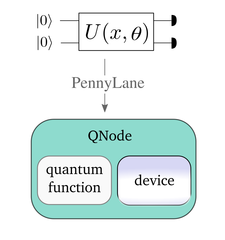
In PennyLane, quantum computations, which involve the execution of one or more quantum circuits, are represented as quantum node objects. A quantum node is used to declare the quantum circuit, and also ties the computation to a specific device that executes it.
QNodes can interface with any of the supported numerical and machine learning libraries—NumPy,
PyTorch, TensorFlow, and
JAX—indicated by providing an optional interface argument
when creating a QNode. Each interface allows the quantum circuit to integrate seamlessly with
library-specific data structures (e.g., NumPy and JAX arrays or Pytorch/TensorFlow tensors) and
optimizers.
By default, QNodes use the NumPy interface. The other PennyLane interfaces are introduced in more detail in the section on interfaces.
Quantum functions
A quantum circuit is constructed as a special Python function, a quantum circuit function, or quantum function in short. For example:
import pennylane as qml

def my_quantum_function(x, y):
    qml.RZ(x, wires=0)
    qml.CNOT(wires=[0,1])
    qml.RY(y, wires=1)
    return qml.expval(qml.PauliZ(1))
Note
PennyLane uses the term wires to refer to a quantum subsystem—for most devices, this corresponds to a qubit. For continuous-variable devices, a wire corresponds to a quantum mode.
Quantum functions are a restricted subset of Python functions, adhering to the following constraints:
The quantum function accepts classical inputs, and consists of quantum operators or sequences of operators called Templates.
The function can contain classical flow control structures such as
forloops orifstatements.The quantum function must always return either a single or a tuple of measurement values, by applying a measurement function to the qubit register. The most common example is to measure the expectation value of a qubit observable or continuous-value observable.
Note
Quantum functions are evaluated on a device from within a QNode.
Defining a device
To run—and later optimize—a quantum circuit, one needs to first specify a computational device.
The device is an instance of the Device
class, and can represent either a simulator or hardware device. They can be
instantiated using the device loader.
dev = qml.device('default.qubit', wires=2, shots=1000)
PennyLane offers some basic devices such as the 'default.qubit', 'default.mixed', lightning.qubit,
'default.gaussian', and 'default.clifford' simulators; additional devices can be installed as plugins
(see available plugins for more details). Note that the
choice of a device significantly determines the speed of your computation, as well as
the available options that can be passed to the device loader.
Note
For example, check out the 'lightning.gpu'
plugin,
which is a fast state-vector simulator offloading to the NVIDIA cuQuantum SDK for GPU accelerated circuit simulation.
Note
For details on saving device configurations, please visit the configurations page.
Device options
When loading a device, the name of the device must always be specified. Further options can then be passed as keyword arguments, and can differ based on the device. For a plugin device, refer to the plugin documentation for available device options.
The two most important device options are the wires and shots arguments.
Wires
The wires argument can be an integer that defines the number of wires
that you can address by consecutive integer labels 0, 1, 2, ....
dev = qml.device('default.qubit', wires=3)
Alternatively, you can use custom labels by passing an iterable that contains unique labels for the subsystems:
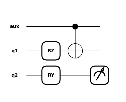
dev_unique_wires = qml.device('default.qubit', wires=['aux', 'q1', 'q2'])
In the quantum function you can now use your own labels to address wires:
def my_quantum_function(x, y):
    qml.RZ(x, wires='q1')
    qml.CNOT(wires=['aux' ,'q1'])
    qml.RY(y, wires='q2')
    return qml.expval(qml.PauliZ('q2'))
Allowed wire labels can be of any type that is hashable, which allows two wires to be uniquely distinguished.
Note
Some devices, such as hardware chips, may have a fixed number of wires.
The iterable of labels passed to the device’s wires
argument must match this expected number of wires.
Warning
In order to support wire labels of any hashable type, integers and 0-d arrays are considered different.
For example, running qml.RX(1.1, qml.numpy.array(0)) on a device initialized with wires=[0]
will fail because qml.numpy.array(0) does not exist in the device’s wire map.
Shots
The shots argument is an integer that defines how many times the circuit should be evaluated (or “sampled”)
to estimate statistical quantities. On some supported simulator devices, shots=None computes
measurement statistics exactly.
Note that this argument can be temporarily overwritten when a QNode is called. For example, my_qnode(shots=3)
will temporarily evaluate my_qnode using three shots. This is a feature of each QNode and it is not
necessary to manually implement the shots keyword argument of the quantum function.
It is sometimes useful to retrieve the result of a computation for different shot numbers without evaluating a QNode several times (“shot batching”). Batches of shots can be specified by passing a list of integers, allowing measurement statistics to be course-grained with a single QNode evaluation.
Consider
>>> shots_list = [5, 10, 1000]
>>> dev = qml.device("default.qubit", wires=2, shots=shots_list)
When QNodes are executed on this device, a single execution of 1015 shots will be submitted. However, three sets of measurement statistics will be returned; using the first 5 shots, second set of 10 shots, and final 1000 shots, separately.
For example:
@qml.qnode(dev)
def circuit(x):
    qml.RX(x, wires=0)
    qml.CNOT(wires=[0, 1])
    return qml.expval(qml.PauliZ(0) @ qml.PauliX(1)), qml.expval(qml.PauliZ(0))
Executing this, we will get an output of shape (3, 2):
>>> results = circuit(0.5)
>>> results
((array(0.6), array(1.)),
 (array(-0.4), array(1.)),
 (array(0.048), array(0.902)))
We can index into this tuple and retrieve the results computed with only 5 shots:
>>> results[0]
(array(0.6), array(1.))
Creating a quantum node
Together, a quantum function and a device are used to create a quantum node or
QNode object, which wraps the quantum function and binds it to the device.
A QNode can be explicitly created as follows:
circuit = qml.QNode(my_quantum_function, dev_unique_wires)
The QNode can be used to compute the result of a quantum circuit as if it was a standard Python function. It takes the same arguments as the original quantum function:
>>> circuit(np.pi/4, 0.7)
tensor(0.764, requires_grad=True)
To view the quantum circuit given specific parameter values, we can use the draw()
transform,
>>> print(qml.draw(circuit)(np.pi/4, 0.7))
aux: ───────────╭●─┤
 q1: ──RZ(0.79)─╰X─┤
 q2: ──RY(0.70)────┤  <Z>
or the draw_mpl() transform:
>>> import matplotlib.pyplot as plt
>>> qml.drawer.use_style("black_white")
>>> fig, ax = qml.draw_mpl(circuit)(np.pi/4, 0.7)
>>> plt.show()
The QNode decorator
A more convenient—and in fact the recommended—way for creating QNodes is the provided
qnode decorator. This decorator converts a Python function containing PennyLane quantum
operations to a QNode circuit that will run on a quantum device.
Note
The decorator completely replaces the Python-based quantum function with
a QNode of the same name—as such, the original
function is no longer accessible.
For example:
dev = qml.device('default.qubit', wires=2)

@qml.qnode(dev)
def circuit(x):
    qml.RZ(x, wires=0)
    qml.CNOT(wires=[0,1])
    qml.RY(x, wires=1)
    return qml.expval(qml.PauliZ(1))

result = circuit(0.543)
Parameter Broadcasting in QNodes
Depending on the quantum operations used, a QNode may support execution at multiple parameters simultaneously:
>>> x = np.array([0.543, 1.234])
>>> result = circuit(x)
>>> result
tensor([0.85616242, 0.33046511], requires_grad=True)
Note that we are passing in a 1-dimensional array of parameters to the circuit() QNode defined above, which takes a single parameter and returns a single expectation value. As the input is now an array, the output is also an array, with each element the expectation value of the corresponding input element.
This is called parameter broadcasting (as for, say, NumPy functions executed along an axis) or parameter batching (as in the application of a function to a batch of parameters in machine learning).
In addition to a more flexible execution syntax, broadcasting can yield performance boosts
compared to the separate execution of the QNode for each parameter setting. Whether or not this is
the case depends on quite a few details, but in particular for (at most) moderately sized circuits
(\(\lesssim 20\) wires) with a moderate number of parameters (\(\lesssim 200\)) executed
on a classical simulator, one can expect to benefit from broadcasting.
See the QNode documentation for usage details.
Many standard quantum operators support broadcasting; see the corresponding attribute
supports_broadcasting for a list. The
Operator documentation contains implementation details
and a guide to make custom operators compatible with broadcasting.
Broadcasting can be used with any device, but will usually only yield performance upgrades for
devices like "default.qubit" that indicate that they support it:
>>> cap = dev.capabilities()
>>> cap["supports_broadcasting"]
True
Other devices separate the parameters and execute the QNode sequentially.
Importing circuits from other frameworks
PennyLane supports creating customized PennyLane templates imported from other
frameworks. By loading your existing quantum code as a PennyLane template, you
add the ability to perform analytic differentiation, and interface with machine
learning libraries such as PyTorch and TensorFlow. Currently, QuantumCircuit
objects from Qiskit, OpenQASM files, pyQuil programs, and Quil files can
be loaded by using the following functions:
Converts a Qiskit QuantumCircuit into a PennyLane quantum function. Loads quantum circuits from a QASM string using the converter in the PennyLane-Qiskit plugin. Loads quantum circuits from a QASM file using the converter in the PennyLane-Qiskit plugin. Loads pyQuil Program objects by using the converter in the PennyLane-Rigetti plugin. Loads quantum circuits from a Quil string using the converter in the PennyLane-Rigetti plugin. Loads quantum circuits from a Quil file using the converter in the PennyLane-Rigetti plugin.
Note
To use these conversion functions, the latest version of the PennyLane-Qiskit and PennyLane-Rigetti plugins need to be installed.
Objects for quantum circuits can be loaded outside or directly inside of a
QNode. Circuits that contain unbound parameters are also
supported. Parameter binding may happen by passing a dictionary containing the
parameter-value pairs.
Once a PennyLane template has been created from such a quantum circuit, it can
be used similarly to other templates in PennyLane. One important thing to note
is that custom templates must always be executed
within a QNode (similar to pre-defined templates).
Note
Certain instructions that are specific to the external frameworks might be ignored when loading an external quantum circuit. Warning messages will be emitted for ignored instructions.
The following is an example of loading and calling a parametrized Qiskit QuantumCircuit object
while using the QNode decorator:
from qiskit import QuantumCircuit
from qiskit.circuit import Parameter
import numpy as np

dev = qml.device('default.qubit', wires=2)

theta = Parameter('θ')

qc = QuantumCircuit(2)
qc.rz(theta, [0])
qc.rx(theta, [0])
qc.cx(0, 1)

@qml.qnode(dev)
def quantum_circuit_with_loaded_subcircuit(x):
    qml.from_qiskit(qc)({theta: x})
    return qml.expval(qml.PauliZ(0))

angle = np.pi/2
result = quantum_circuit_with_loaded_subcircuit(angle)
Furthermore, loaded templates can be used with any supported device, any number of times.
For instance, in the following example a template is loaded from a QASM string,
and then used multiple times on the forest.qpu device provided by PennyLane-Rigetti:
import pennylane as qml

dev = qml.device('forest.qpu', wires=2)

hadamard_qasm = 'OPENQASM 2.0;' \
                'include "qelib1.inc";' \
                'qreg q[1];' \
                'h q[0];'

apply_hadamard = qml.from_qasm(hadamard_qasm)

@qml.qnode(dev)
def circuit_with_hadamards():
    apply_hadamard(wires=[0])
    apply_hadamard(wires=[1])
    qml.Hadamard(wires=[1])
    return qml.expval(qml.PauliX(0)), qml.expval(qml.PauliX(1))

result = circuit_with_hadamards()